Databases, Data Warehouses and Data Types Explained for Analysts

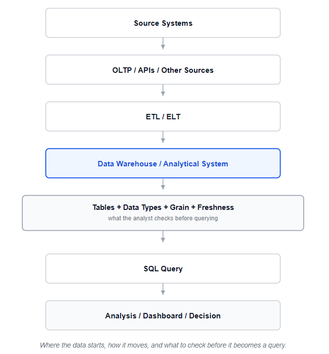
Most explanations of databases are written for the people who build and maintain them, which means they spend most of their length on things an analyst never touches: indexing strategy, replication, server configuration. That's the wrong depth for this job. What actually matters before writing SQL is a working mental model: why your query sometimes hits a live production system and sometimes hits a separate copy of the data, why that copy isn't always perfectly current, what a column's data actually is versus what its name implies, and why one row in one table might not mean what you assume it means once you join it to another.

This guide covers exactly that layer, no server administration, no engineering depth you won't use, just the concepts that explain what you're looking at before you write the query that touches it.

The 8 Database Concepts You Actually Need as a Data Analyst

Together, these eight answer the same underlying question from different angles: what am I actually looking at, before I write a line of SQL against it? Get comfortable with these and SQL syntax will make noticeably more sense on first contact, since you'll already understand why the data is shaped the way it is.

1. What a database actually is

A database is a structured place data lives, organised into tables, each table holding rows and columns, much like the spreadsheet mental model you likely already have. What makes it a database rather than a spreadsheet is that many people and systems can read and write to it at once, reliably, without corrupting each other's changes. A food delivery app's database is being written to constantly: a new order here, a status update there, hundreds of times a second during a lunch rush.

That constant read-and-write activity is the detail that explains almost everything else in this guide.

2. OLTP vs OLAP

OLTP, online transaction processing, describes a database built for exactly the food delivery scenario above: many small, fast operations happening constantly, an order placed, a payment recorded, a delivery status updated. These systems are optimised for writing data quickly and reliably, one transaction at a time.

OLAP, online analytical processing, is optimised for a very different workload: fewer, much larger analytical queries, scanning millions of rows to compute a monthly total rather than writing one row at a time. This is the kind of analytical workload many analysts encounter day to day.

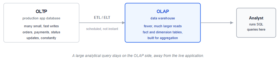
These two workloads put genuinely different demands on a system. Google Cloud's own engineering team describes this same split: OLTP systems are optimised for high-volume, low-latency transactions using row-oriented storage, while analytical workloads need rapid aggregations and scans across large datasets, which is traditionally why separate data warehouses exist at all. A large analytical query scanning millions of rows can slow down a live application if it runs against the same database handling real customer orders. In many organisations, analysts query an analytical system or warehouse rather than the live OLTP database, specifically to avoid that conflict. That said, this isn't universal: at smaller companies, or for smaller ad-hoc questions, analysts sometimes query production systems or a read replica directly. The concept that matters is knowing which kind of system you're pointed at, not a hard rule about who's allowed to touch what.

3. What a data warehouse actually is

A data warehouse is a system designed to consolidate and serve data for analytical workloads, typically separate from the systems handling live transactions. It pulls data from one or more source systems, often several OLTP databases plus other sources like marketing platforms or support ticket systems, into one place built for querying.

A common warehouse modelling pattern uses fact tables, holding transactional numbers, and dimension tables, holding descriptive attributes, connected by relationships. This isn't the only way a warehouse can be structured, but it's common enough to be worth recognising, and it's the same pattern covered in the Power BI for Beginners tutorial, because it suits the read-heavy, aggregation-heavy queries a warehouse is built to answer quickly, in a way that doesn't suit an OLTP database's write-heavy job.

4. How data gets into the warehouse: ETL vs ELT

Getting data from source systems into a warehouse is usually called ETL or ELT, and the difference is in the order of operations:

ETL: Extract, then Transform, then Load. Data is cleaned and reshaped before it ever reaches the warehouse.

ELT: Extract, then Load, then Transform. Raw data lands in the warehouse first, and the cleaning or reshaping happens afterward, inside the warehouse itself.

The important difference for an analyst isn't the acronym order, it's knowing that in modern analytical systems, transformations can often happen inside the warehouse after the raw data has already been loaded, which means a table you're querying might be an intermediate, not-yet-fully-cleaned version of the data, depending on where it sits in that pipeline. Google Cloud describes ELT as its own recommended pattern for exactly this reason: loading raw data first lets any SQL-literate person build transformations using the warehouse's own processing power, rather than requiring a separate transformation step before anything lands. If a table's numbers look inconsistent with a more polished dashboard elsewhere, checking where that table sits in the ETL or ELT process is a reasonable first step.

5. Structured, semi-structured, and unstructured data

Most of what an analyst queries directly is structured data: rows and columns, a defined schema, the kind SQL was built for. But two other categories show up often enough to be worth naming.

Semi-structured data has some organisation but doesn't fit neatly into fixed columns, the most common example being JSON, a nested format frequently used for things like API responses or event logs. A single column in an otherwise normal table might contain an entire JSON object as text, and querying inside it usually needs specific JSON functions rather than a plain column reference.

Unstructured data has no predefined organisation at all, free text, images, audio, PDF documents. Analysts touch this less directly, but it's increasingly common as an input to something that eventually becomes structured, a support call transcribed to text and then categorised into a clean column, for instance.

6. The data types you'll actually encounter in SQL

The section above covers data structure, rows and columns versus JSON versus free text. This is a different, narrower question: once you're looking at an actual column in an actual table, what type of value does it hold?

You don't need to memorise every type system quirk across every database engine to work with this list day to day, though the exact set of types varies by engine; PostgreSQL's data type documentation is a useful reference for how much detail sits underneath what looks like a short list. What matters more for daily work is the habit underneath it:

A column's name does not guarantee its actual data type.

A column called amount that was actually loaded as text, or a column called metadata that's secretly a JSON blob, behaves very differently in a query than its name implies. Checking a column's actual data type before building a calculation on it, the same habit that matters in Excel and Pandas, matters here too, for the same reason: a numeric-looking value stored as text can behave differently from a true numeric column and may cause errors, implicit conversions, or unexpected results depending on the database system.

7. What does one row actually represent?

This is table grain, and it's one of the most practically important concepts in this entire guide, because getting it wrong is one of the easiest ways to silently produce a wrong number.

Orders

One row = one order.

Order Items

One row = one product within an order.

Notice that order 101 appears twice in Order Items, once per product in that order. If an analyst joins Orders to Order Items without understanding that grain shift, order 101's row gets duplicated in the joined result, once for each item. Summing an order-level revenue column after that join without accounting for the duplication will overcount revenue for every multi-item order, quietly and without any error message.

Before joining two tables, know what one row represents in each table. That single habit prevents a large share of the most common SQL mistakes analysts make early on.

8. How fresh is the data?

Freshness is a specific, checkable question, not a vague sense that "warehouses are slow." It depends on where in the pipeline you're looking:

• Source-system data, inside the live OLTP application, is as current as the moment someone last performed the action.

• Warehouse data reflects whatever the last completed ETL or ELT run loaded, which could be minutes, hours, or a full day behind, depending on how that specific pipeline is scheduled.

• Refresh schedules vary by pipeline and by company, from hourly loads to nightly batch jobs to genuinely near-real-time streaming for specific high-priority use cases. There's no single universal answer, which is exactly why it's worth checking rather than assuming.

Not every warehouse is delayed, and not every OLTP system is instantaneous from an analyst's point of view either; the only safe assumption is that you should know the refresh schedule for whatever you're querying, rather than guessing. If a dashboard number looks different from what someone sees in the live application, check data freshness and pipeline timing before assuming the SQL is wrong.

Before you write the query, check these 5 things

1. Where does this data come from? Knowing the source system tells you what the data was originally designed to capture, and what it might be missing.

2. Am I querying OLTP, OLAP, a warehouse, or another analytical source? This affects both the performance impact of your query and how current the results are.

3. When was the data last refreshed? A number that looks wrong is sometimes just a number that's current as of an earlier pipeline run, not an error in your query.

4. What is the actual data type of the columns I need? Check rather than assume, especially for anything you're about to sum, average, or filter numerically.

5. What does one row represent? Confirm this for every table involved before joining, especially before summing anything across the join.

Running through this list takes under a minute once it's a habit, and it can prevent many of the common mistakes below.

Common mistakes

• Assuming warehouse data is live. ETL and ELT pipelines run on a schedule, and a mismatch between a dashboard number and what's visible in the live app is usually a timing issue, not an error in either system.

• Treating "database" and "table" as interchangeable. A database is the whole structured system; a table is one structured object inside it. The distinction matters once you start writing queries that join several tables together.

• Not checking data types before calculating. This is the same lesson that shows up in Excel and Pandas, and it starts here, at the schema level, before either tool ever sees the data.

• Joining tables without checking their grain first. This is how an innocent-looking join quietly duplicates rows and inflates a sum, without any error to flag it.

• Querying a live transactional system for heavy analysis without realising the impact. A large analytical query against a production database can slow it down for real users, which is one of the main reasons analytical systems and warehouses exist as a separate option.

• Not asking where semi-structured data actually lives. A JSON column hiding inside an otherwise normal-looking table is easy to miss until a query against it returns something unexpected.

Where to go from here

This guide covers the analyst-specific slice of a much bigger topic; for a broader look at what a database management system actually does, the existing What is DBMS article covers that ground in more general terms.

The natural next step from here is the SQL for Data Analysts guide, since most of what's covered above exists to explain why the data looks the way it does once you start writing real queries against it. If you'd rather start writing SQL immediately, Your First 10 SQL Queries puts these concepts to work against a real table, and SQL CASE statements picks up shortly after that, once filtering and sorting feel comfortable and it's time to add business logic inside a query.

The fact and dimension table pattern mentioned above shows up again, in more depth, once you start building in Power BI; Power BI data modeling walks through a five-table sales model built on exactly this structure.