10 SQL Patterns Every Data Analyst Should Recognize

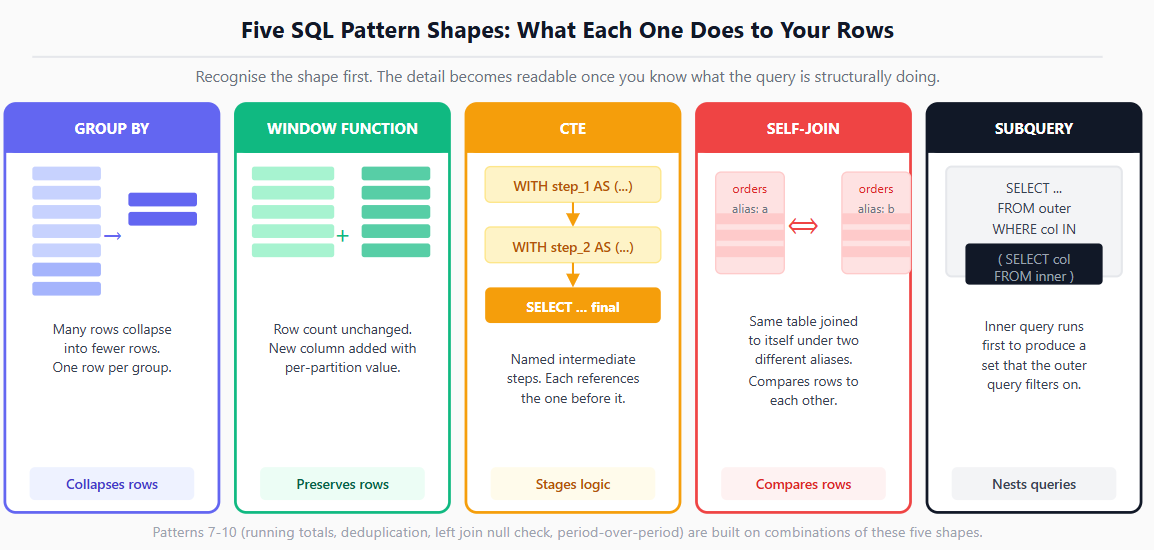
SQL has a relatively small surface area of syntax. The keywords are not many, the grammar is consistent, and a reasonable analyst can learn to write basic queries in a few days. What takes longer is developing the ability to look at a query you have never seen before and immediately understand what it is doing and why it is shaped that way.

That ability comes from pattern recognition. Experienced analysts do not read queries word by word. They read them shape by shape, the same way an experienced reader does not process individual letters. They see a window function and know it is computing something relative to a group without collapsing the rows. They see a self-join and know it is comparing rows within the same table. They see a correlated subquery and understand immediately what the relationship is between the inner and outer queries.

This article covers ten SQL patterns that appear constantly in real analytical work. For each one: what it does, what the shape looks like, a practical analyst example, and what to watch for when you encounter it. The database used for examples is a standard e-commerce schema with orders, customers, products, and events tables, which makes the patterns transferable to any domain with minimal translation.

The running example schema

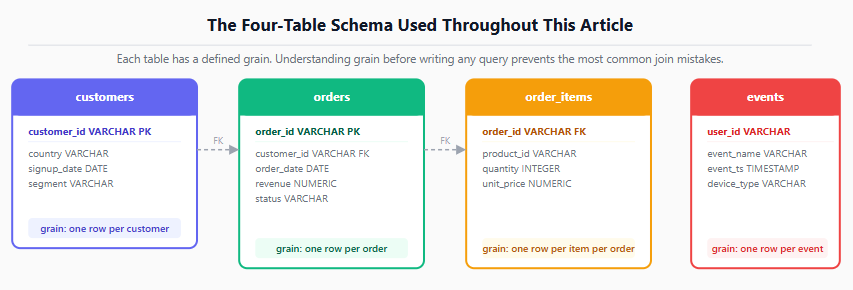
All ten patterns use variations of these four tables:

sql

-- customers: one row per customer
customer_id   VARCHAR
country       VARCHAR
signup_date   DATE
segment       VARCHAR   -- 'free', 'pro', 'enterprise'

-- orders: one row per order
order_id      VARCHAR
customer_id   VARCHAR
order_date    DATE
revenue       NUMERIC
status        VARCHAR   -- 'completed', 'refunded', 'pending'

-- order_items: one row per product per order
order_id      VARCHAR
product_id    VARCHAR
quantity      INTEGER
unit_price    NUMERIC

-- events: one row per user action
user_id       VARCHAR
event_name    VARCHAR
event_ts      TIMESTAMP
device_type   VARCHAR

This schema is simple enough to follow without domain expertise and realistic enough that every pattern in this article is drawn directly from the kinds of questions these tables actually produce.

Pattern 1: Aggregation with GROUP BY

What it solves: Summarising a large table into one row per group, with a calculated value for each group.

This is the most fundamental analytical pattern in SQL. Every pivot table, every summary report, every dashboard metric that involves a breakdown by dimension is a GROUP BY underneath.

sql

-- Total revenue and order count by country, completed orders only
SELECT
    c.country,
    COUNT(DISTINCT o.order_id)      AS total_orders,
    SUM(o.revenue)                  AS total_revenue,
    ROUND(AVG(o.revenue), 2)        AS avg_order_value
FROM orders o
JOIN customers c ON o.customer_id = c.customer_id
WHERE o.status = 'completed'
GROUP BY c.country
ORDER BY total_revenue DESC;

What to watch for: The WHERE clause filters rows before grouping. The HAVING clause (not shown here) filters after grouping. This distinction matters when you want to exclude groups with low volume: HAVING COUNT(*) >= 10 removes groups with fewer than ten orders from the result, which WHERE cannot do because the group does not exist yet at that point in execution.

Also watch the SELECT list: every column that is not inside an aggregate function (SUM, COUNT, AVG, MAX, MIN) must appear in the GROUP BY. If it does not, most databases will raise an error or produce non-deterministic results.

Pattern 2: Window Functions

What it solves: Computing a value relative to a partition of rows, without collapsing those rows into one.

This is the pattern that separates analysts who can answer complex ranking and running-total questions from those who cannot. Window functions add a calculated column to every row, computed across a defined window of rows, without changing the number of rows in the result.

sql

-- Rank orders by revenue within each country
-- and compute each order's share of that customer's total revenue
SELECT
    o.order_id,
    o.customer_id,
    c.country,
    o.revenue,
    RANK() OVER (
        PARTITION BY c.country
        ORDER BY o.revenue DESC
    )                                               AS revenue_rank_in_country,
    ROUND(
        o.revenue / SUM(o.revenue) OVER (
            PARTITION BY o.customer_id
        ) * 100, 1
    )                                               AS pct_of_customer_total
FROM orders o
JOIN customers c ON o.customer_id = c.customer_id
WHERE o.status = 'completed';

The anatomy of a window function is always: FUNCTION() OVER (PARTITION BY ... ORDER BY ...). The PARTITION BY defines the group the function operates within. The ORDER BY inside OVER defines the ordering within that partition, which matters for ranking and running calculations. Neither collapse rows.

What to watch for: RANK() leaves gaps after ties (ranks 1, 1, 3). DENSE_RANK() does not (ranks 1, 1, 2). ROW_NUMBER() assigns a unique number regardless of ties. Choosing the wrong one produces subtly wrong results in ranking-based analysis. The PostgreSQL window functions documentation provides a precise reference for each function's behaviour.

Pattern 3: CTEs (Common Table Expressions)

What it solves: Breaking a complex query into named, readable steps that reference each other in sequence.

A CTE is not a performance optimisation in most databases. It is a readability and maintainability tool. It lets you name an intermediate result, then reference that name later in the same query, exactly as you would define a variable before using it in code.

sql

-- Step 1: customers who placed more than 3 completed orders
-- Step 2: their average order value
-- Step 3: compare to overall average

WITH high_value_customers AS (
    SELECT
        customer_id,
        COUNT(order_id)     AS order_count,
        SUM(revenue)        AS total_revenue
    FROM orders
    WHERE status = 'completed'
    GROUP BY customer_id
    HAVING COUNT(order_id) > 3
),

overall_avg AS (
    SELECT AVG(revenue) AS avg_revenue
    FROM orders
    WHERE status = 'completed'
)

SELECT
    h.customer_id,
    h.order_count,
    h.total_revenue,
    ROUND(h.total_revenue / h.order_count, 2)   AS avg_order_value,
    o.avg_revenue                                AS overall_avg,
    ROUND(
        (h.total_revenue / h.order_count) - o.avg_revenue,
    2)                                           AS diff_from_overall
FROM high_value_customers h
CROSS JOIN overall_avg o
ORDER BY avg_order_value DESC;

What to watch for: CTEs are defined once and can be referenced multiple times in the same query. Chaining too many CTEs (more than five or six) can make the query harder to follow rather than easier. If a CTE is only used once and is short, an inline subquery or a derived table is often cleaner. CTEs are not materialised by default in most databases (PostgreSQL, BigQuery, Snowflake, Redshift), meaning the engine may re-execute the CTE each time it is referenced, though this is engine-specific and worth verifying when performance matters.

Pattern 4: Self-Join

What it solves: Comparing rows within the same table to each other, most commonly for finding pairs, sequences, or gaps.

A self-join treats the same table as if it were two different tables with different aliases. The most common analyst uses are: finding customers who placed orders in two specific periods, comparing a metric to its previous period, and identifying duplicates.

sql

-- Find customers who placed an order in both Jan 2026 and Feb 2026
-- (month-over-month retention check)

SELECT DISTINCT jan.customer_id
FROM orders jan
JOIN orders feb
    ON jan.customer_id = feb.customer_id
   AND DATE_TRUNC('month', jan.order_date) = '2026-01-01'
   AND DATE_TRUNC('month', feb.order_date) = '2026-02-01'
WHERE jan.status = 'completed'
  AND feb.status = 'completed';

What to watch for: Self-joins are easy to write in a way that produces every pair of rows twice, or that includes a row paired with itself. For pair-finding queries, use a.id < b.id to ensure each pair appears once and a row is not paired with itself. For retention queries like the one above, the DISTINCT keyword prevents the same customer appearing multiple times if they placed multiple orders in either month.

Pattern 5: Subquery in WHERE (filtering with a derived set)

What it solves: Filtering the outer query to only rows that match a condition computed by a separate inner query.

This pattern appears whenever the filter condition cannot be expressed as a simple value and instead requires its own aggregation or lookup.

sql

-- Orders placed by customers whose total lifetime revenue exceeds 1000
-- (without pulling total_revenue into a CTE first)

SELECT
    order_id,
    customer_id,
    order_date,
    revenue
FROM orders
WHERE customer_id IN (
    SELECT customer_id
    FROM orders
    WHERE status = 'completed'
    GROUP BY customer_id
    HAVING SUM(revenue) > 1000
)
AND status = 'completed'
ORDER BY order_date;

What to watch for: IN (subquery) and EXISTS (subquery) are different shapes for similar problems. IN tests whether a value belongs to the result of the subquery, while EXISTS tests whether at least one matching row exists. Query optimizers may transform either form, so do not assume one will always be faster than the other. The practical difference depends on the specific engine and its query planner. If the inner query can return NULL values, NOT IN behaves unexpectedly: a single NULL in the inner set causes the outer NOT IN to return no rows, because value NOT IN (... NULL ...) evaluates to unknown rather than false.

Pattern 6: CASE WHEN (conditional column logic)

What it solves: Creating a new column whose value depends on a condition, either as a classification, a bucket, or a conditional aggregate.

CASE WHEN is SQL's if-then-else. It appears in two distinct roles: as a standalone column expression that categorises or labels rows, and inside an aggregate function to create conditional aggregations (sometimes called pivot-style aggregation).

sql

-- Role 1: Classify orders into revenue buckets
SELECT
    order_id,
    revenue,
    CASE
        WHEN revenue >= 500  THEN 'high'
        WHEN revenue >= 100  THEN 'medium'
        ELSE 'low'
    END AS revenue_tier
FROM orders
WHERE status = 'completed';

-- Role 2: Conditional aggregation, one row per customer,
-- separate columns for completed vs refunded revenue
SELECT
    customer_id,
    SUM(CASE WHEN status = 'completed' THEN revenue ELSE 0 END) AS completed_revenue,
    SUM(CASE WHEN status = 'refunded'  THEN revenue ELSE 0 END) AS refunded_revenue,
    COUNT(CASE WHEN status = 'completed' THEN 1 END)            AS completed_orders
FROM orders
GROUP BY customer_id;

What to watch for: In the conditional aggregation pattern, SUM(CASE WHEN ... THEN revenue ELSE 0 END) and SUM(CASE WHEN ... THEN revenue END) behave differently when no rows match: the first returns 0, the second returns NULL. The right choice depends on whether a NULL or a zero is the correct representation of "no matching rows" for your downstream logic.

Pattern 7: Running Totals and Moving Averages

What it solves: Computing a cumulative or rolling value as rows are traversed in order.

This is a specific application of window functions but common enough to warrant its own pattern. Running totals accumulate across all prior rows in the partition. Moving averages smooth a metric over a rolling window of N preceding rows.

sql

-- Monthly revenue with running total and 3-month moving average
-- PostgreSQL syntax; adapt DATE_TRUNC and date arithmetic for other engines

WITH monthly AS (
    SELECT
        DATE_TRUNC('month', order_date)     AS month,
        SUM(revenue)                        AS monthly_revenue
    FROM orders
    WHERE status = 'completed'
    GROUP BY 1
)

SELECT
    month,
    monthly_revenue,
    SUM(monthly_revenue) OVER (
        ORDER BY month
        ROWS BETWEEN UNBOUNDED PRECEDING AND CURRENT ROW
    )                                       AS running_total,
    ROUND(AVG(monthly_revenue) OVER (
        ORDER BY month
        ROWS BETWEEN 2 PRECEDING AND CURRENT ROW
    ), 2)                                   AS moving_avg_3m
FROM monthly
ORDER BY month;

What to watch for: The frame clause (ROWS BETWEEN ...) controls which rows are included in the window. ROWS BETWEEN UNBOUNDED PRECEDING AND CURRENT ROW gives a true running total from the beginning of the partition. ROWS BETWEEN 2 PRECEDING AND CURRENT ROW gives the current row plus the two rows before it, producing a three-period moving average. Without a frame clause, the default behaviour varies by function and engine, so always specify it explicitly for running calculations.

Pattern 8: Deduplication with ROW_NUMBER()

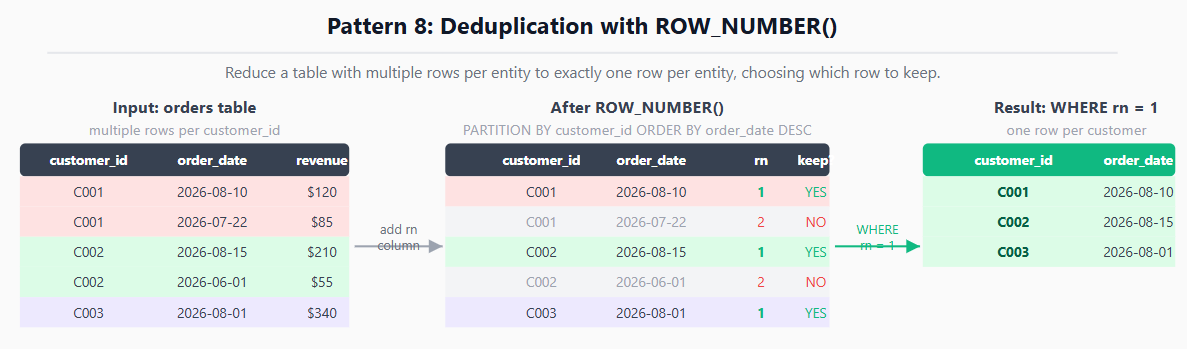
What it solves: Keeping exactly one row per entity from a table that contains duplicates or multiple records per entity, by ranking rows within each group and keeping only rank 1.

This is one of the most practically important patterns in analytics data preparation. Source tables frequently contain multiple records per customer or user because of how events are logged, how snapshots are taken, or how ETL processes work. Before joining or aggregating, you often need to reduce these to one row per entity.

sql

-- Keep only the most recent order per customer
-- (deduplication: one row per customer_id)

WITH ranked AS (
    SELECT
        *,
        ROW_NUMBER() OVER (
            PARTITION BY customer_id
            ORDER BY order_date DESC
        ) AS rn
    FROM orders
    WHERE status = 'completed'
)

SELECT
    customer_id,
    order_id,
    order_date,
    revenue
FROM ranked
WHERE rn = 1;

What to watch for: ROW_NUMBER() assigns a unique rank even when rows are tied (for example, two orders on the same date). If ties exist and the choice between tied rows is not arbitrary, you need a tiebreaker in the ORDER BY (for example, ORDER BY order_date DESC, order_id DESC). If you want all tied rows rather than one, use RANK() = 1 instead of ROW_NUMBER() = 1, noting that RANK produces ties and ROW_NUMBER does not.

Pattern 9: Left Join with NULL Check (finding what is missing)

What it solves: Identifying rows in one table that have no matching row in another table.

This pattern is the SQL equivalent of "show me everything in set A that is not in set B." It appears in churn analysis (customers who never ordered), gap analysis (days with no events), and data quality checks (orders with no matching customer record).

sql

-- Customers who signed up in the last 90 days but have never placed an order

SELECT
    c.customer_id,
    c.signup_date,
    c.segment
FROM customers c
LEFT JOIN orders o
    ON c.customer_id = o.customer_id
   AND o.status = 'completed'
WHERE o.order_id IS NULL
  AND c.signup_date >= CURRENT_DATE - INTERVAL '90 days';

The LEFT JOIN returns all rows from customers and matches from orders where they exist. Where no match exists, the orders columns are NULL. The WHERE o.order_id IS NULL then keeps only the rows where no match was found.

What to watch for: The join condition and the WHERE condition interact carefully here. If the filter o.status = 'completed' were placed in the WHERE clause instead of the JOIN condition, it would convert the LEFT JOIN into an INNER JOIN, eliminating customers who have only pending or refunded orders from the result. Conditions that are part of the join logic belong in the ON clause, not the WHERE clause, when using a LEFT JOIN.

Pattern 10: Period-over-Period Comparison

What it solves: Comparing a metric from the current period to the same metric from a prior period in a single query, without a separate query for each period.

This is one of the most requested patterns in business analytics: revenue this month versus last month, active users this week versus last week, conversion this quarter versus last quarter. There are two main approaches: self-join on period, and conditional aggregation with CASE WHEN.

One important caveat for live current-month reporting: if you run this query mid-month, the current-month bucket captures only days elapsed so far, while the prior-month bucket captures the full previous month. That is an apples-to-oranges comparison. For a fair comparison, either compare the same number of elapsed days in both periods, or use this pattern specifically for completed-period reporting where the current month is already closed.

sql

-- Month-to-date revenue vs previous full month revenue
-- Note: run mid-month, this_month_revenue covers only days elapsed
-- so far, not a full month. Compare equivalent windows for a fair MoM.
-- Using conditional aggregation (no self-join needed)

SELECT
    SUM(CASE
            WHEN DATE_TRUNC('month', order_date) =
                 DATE_TRUNC('month', CURRENT_DATE)
            THEN revenue ELSE 0
        END)                                             AS this_month_revenue,
    SUM(CASE
            WHEN DATE_TRUNC('month', order_date) =
                 DATE_TRUNC('month', CURRENT_DATE) - INTERVAL '1 month'
            THEN revenue ELSE 0
        END)                                             AS last_month_revenue,
    SUM(CASE
            WHEN DATE_TRUNC('month', order_date) =
                 DATE_TRUNC('month', CURRENT_DATE)
            THEN revenue ELSE 0
        END) -
    SUM(CASE
            WHEN DATE_TRUNC('month', order_date) =
                 DATE_TRUNC('month', CURRENT_DATE) - INTERVAL '1 month'
            THEN revenue ELSE 0
        END)                                             AS revenue_change,
    ROUND(
        (SUM(CASE WHEN DATE_TRUNC('month', order_date) =
                       DATE_TRUNC('month', CURRENT_DATE)
                  THEN revenue ELSE 0 END) -
         SUM(CASE WHEN DATE_TRUNC('month', order_date) =
                       DATE_TRUNC('month', CURRENT_DATE) - INTERVAL '1 month'
                  THEN revenue ELSE 0 END))
        / NULLIF(
            SUM(CASE WHEN DATE_TRUNC('month', order_date) =
                          DATE_TRUNC('month', CURRENT_DATE) - INTERVAL '1 month'
                     THEN revenue ELSE 0 END),
        0) * 100, 1
    )                                                    AS pct_change
FROM orders
WHERE status = 'completed'
  AND order_date >= DATE_TRUNC('month', CURRENT_DATE) - INTERVAL '1 month';

What to watch for: NULLIF(denominator, 0) in the percentage change calculation prevents a division-by-zero error when last month's revenue is zero. Without it, the query fails or returns NULL depending on the engine. The INTERVAL '1 month' syntax works in PostgreSQL and Snowflake; BigQuery uses INTERVAL 1 MONTH (integer, no quotes around the unit). Always verify date arithmetic syntax against your specific engine's documentation.

Also watch the time-window mismatch: when run mid-month, DATE_TRUNC('month', CURRENT_DATE) captures only the days elapsed in the current month, while the prior-month condition captures the entire previous month. Comparing month-to-date revenue against a completed prior month will almost always show a decline that reflects the shorter window, not business performance. For a valid comparison, restrict both periods to the same number of elapsed days, or run this pattern only on completed months.

How these ten patterns combine in practice

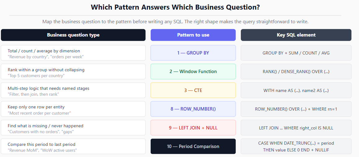
Real analytical queries are rarely a single pattern in isolation. A query that answers "which countries saw the largest month-over-month revenue growth last quarter, excluding countries with fewer than 50 orders?" combines Pattern 1 (GROUP BY), Pattern 6 (CASE WHEN for period logic), Pattern 10 (period-over-period), and Pattern 3 (CTE to stage the steps readably).

Recognising the individual patterns first makes the combined query readable. The analyst who can identify the CTE structure, spot the window function inside it, and read the LEFT JOIN NULL check at the end is reading the query the same way the author wrote it: as a composition of known shapes, not as a wall of text.

When you encounter an unfamiliar query, identify the pattern before reading the detail. What is the outermost shape? Is there a CTE chain? Are there window functions or subqueries? Answering those structural questions first makes the rest of the query easier to parse.

Common mistakes with these patterns

Using WHERE instead of HAVING to filter aggregated results. WHERE runs before aggregation. HAVING runs after. If you want to exclude groups below a threshold, it must be in HAVING, not WHERE.

Confusing RANK(), DENSE_RANK(), and ROW_NUMBER(). All three produce a number per row within a partition. Only ROW_NUMBER guarantees uniqueness. RANK leaves gaps after ties. DENSE_RANK does not. Using the wrong one in a deduplication query keeps more or fewer rows than intended.

Putting LEFT JOIN filter conditions in WHERE instead of ON. A filter in WHERE turns a LEFT JOIN into an INNER JOIN. Conditions that determine whether a row matches belong in ON. Conditions that filter the final result belong in WHERE.

Not handling NULL in NOT IN subqueries. If the inner result set of a NOT IN can contain NULL, no outer rows will match. Use NOT EXISTS or add WHERE inner_column IS NOT NULL inside the subquery to avoid this.

Missing the frame clause in window functions. Without an explicit ROWS BETWEEN or RANGE BETWEEN, the default frame varies by function and engine. For running totals and moving averages, always specify the frame explicitly.

Writing period-over-period comparisons without NULLIF in the denominator. A zero prior-period value causes a division-by-zero error or NULL result. Always wrap the denominator in NULLIF(denominator, 0).

Before writing your next query: a checklist

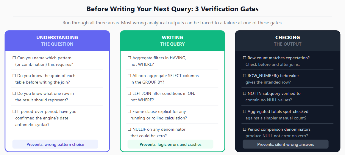
Understanding the question

• Can you name which of the ten patterns (or combination) this question requires?

• Do you know the grain of each table you are joining before writing the join?

• Do you know what one row in the result should represent?

Writing the query

• Are aggregate filter conditions in HAVING, not WHERE?

• Is every non-aggregate column in the SELECT also in the GROUP BY?

• Do LEFT JOIN filter conditions belong in ON, not WHERE?

• Is the frame clause explicitly specified for any running or rolling window calculation?

• Is NULLIF used wherever a denominator could be zero?

Checking the output

• Does the row count match your expectation? Check before and after joins.

• If you used ROW_NUMBER() for deduplication, did you verify the tiebreaker produces the row you intended to keep?

• If you used NOT IN, did you verify the inner result set cannot contain NULL?

Where to go from here

These ten patterns are the foundation. The SQL for Data Analysts guide covers how to build on them in the context of real analytical workflows, including how queries connect to the broader process of defining metrics, checking data quality, and delivering findings.

For the data layer underneath the queries, understanding how databases and data warehouses actually work explains why queries behave the way they do across different engines. Schema structure, table grain, and data freshness all affect how these patterns perform and what their output actually means.

For analysts applying these patterns in Python, the pandas fundamentals guide maps most of these SQL patterns to their pandas equivalents, which is useful for understanding how the same analytical logic translates across tools. The pandas vs Excel guide also covers when SQL-in-the-warehouse is the right layer for a query versus when pulling data into Python for further transformation makes more sense.