Pandas Basics: DataFrames, Series, Indexing and Filtering

Pandas Basics: DataFrames, Series, Indexing and Filtering

If you've already worked through SQL, Pandas is less a new language than a translation exercise. A SELECT is a column choice. A WHERE clause is a boolean filter. A GROUP BY is a .groupby(). The syntax looks unfamiliar the first time, but the underlying thinking, filter this, aggregate that, join these two things on a key, is exactly what you already practised in SQL. This guide leans into that directly: every core Pandas operation below sits next to the SQL line that does the same job.

The running example is a ride-hailing platform's trip data, one row per completed or cancelled trip, with a driver ID, city, fare, distance, and status. Realistic enough to need real filtering, small enough to keep the code readable.

DataFrame and Series: the two objects everything else builds on

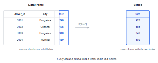
A DataFrame is a table: rows and columns, exactly like a SQL result set. A Series is a single column from that table, with its own index attached. Every column you pull out of a DataFrame is a Series, and understanding that distinction early prevents a lot of confusing error messages later, since some operations expect a DataFrame and others expect a Series, and Pandas won't always tell you clearly which one you handed it.

Loading and looking at your data

python

import pandas as pd

trips = pd.read_csv("trips.csv")
trips.head()
trips.info()

pd.read_csv() loads the file into a DataFrame. head() shows the first five rows, the equivalent of SELECT * FROM trips LIMIT 5. info() shows column names, data types, and how many non-null values each column has, which is worth checking before anything else; a fare column that Pandas read as text rather than a number will silently break every calculation you try to run on it later.

Selecting columns: the SELECT equivalent

python

trips["fare"]                          # one column, returns a Series
trips[["fare", "distance_km"]]         # multiple columns, returns a DataFrame

sql

SELECT fare FROM trips;
SELECT fare, distance_km FROM trips;

The single-bracket version returns a Series; the double-bracket version, a list of column names inside the selector, returns a DataFrame even if it's only one column long. That distinction trips people up constantly, since trips["fare"] and trips[["fare"]] look almost identical but behave differently in later operations that expect one type or the other.

Filtering rows: the WHERE equivalent

python

trips[trips["city"] == "Bangalore"]

sql

SELECT * FROM trips WHERE city = 'Bangalore';

This is boolean indexing, Pandas's core filtering mechanism, and it's worth understanding what's actually happening rather than memorising the syntax. trips["city"] == "Bangalore" produces a Series of True/False values, one per row. Wrapping that Series in trips[...] keeps only the rows where the value is True. Once that clicks, filtering on multiple conditions is the same idea extended:

python

trips[(trips["city"] == "Bangalore") & (trips["status"] == "completed")]

sql

SELECT * FROM trips WHERE city = 'Bangalore' AND status = 'completed';

Where this bites people: using Python's and instead of &, or forgetting the parentheses around each condition. Pandas needs & and | for element-wise boolean logic, not the plain and/or keywords, and without parentheses around each condition, Python's operator precedence reads the expression incorrectly and throws a confusing error rather than a clear one.

loc and iloc: label-based versus position-based access

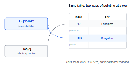
This is the pair that confuses nearly every beginner at least once, and it maps to two different SQL habits.

.loc selects by labels. When you use it with a boolean condition, it feels similar to SQL's WHERE because you're selecting rows based on values.

python

trips.loc[trips["status"] == "cancelled", ["driver_id", "city"]]

sql

SELECT driver_id, city FROM trips WHERE status = 'cancelled';

.iloc selects by integer position, regardless of what the labels are, closer to asking for "the Nth row" than filtering on a value.

python

trips.iloc[0:5, 0:3]     # first 5 rows, first 3 columns, by position

Show Image

There's no clean SQL equivalent for .iloc, because SQL tables are conceptually unordered; asking for "row 3" doesn't mean anything in standard SQL the way it does in a Pandas DataFrame. That's a genuine difference between the two tools, not just a syntax quirk, and it's worth knowing explicitly rather than discovering it by accident.

Where this bites people: using .iloc with a label, or .loc with a plain integer position, and getting a confusing KeyError rather than the row you expected. If your index isn't the default 0, 1, 2… integer index, .loc[3] and .iloc[3] can return completely different rows.

A worked example: which drivers have the most cancellations

The question: identify drivers whose cancellation rate looks unusually high, to flag for a quality review.

python

cancelled = trips[trips["status"] == "cancelled"]
cancellation_counts = cancelled.groupby("driver_id").size()
total_trips = trips.groupby("driver_id").size()
cancellation_rate = (cancellation_counts / total_trips).fillna(0)
cancellation_rate.sort_values(ascending=False).head(10)

sql

SELECT
    driver_id,
    SUM(CASE WHEN status = 'cancelled' THEN 1 ELSE 0 END) * 1.0
        / COUNT(*) AS cancellation_rate
FROM trips
GROUP BY driver_id
ORDER BY cancellation_rate DESC
LIMIT 10;

Both versions do the same thing: filter to cancellations, count by driver, divide by each driver's total trips, and sort. The .groupby() call is doing the same splitting work as SQL's GROUP BY in both queries above. Because cancellation_counts only contains drivers who had at least one cancellation, dividing it by total_trips creates missing values for drivers with zero cancellations. fillna(0) converts those missing rates to the expected zero, and skipping this step is an easy way to lose drivers from your results without any error telling you they're gone.

Common mistakes

• Confusing single brackets and double brackets when selecting columns. df["col"] is a Series; df[["col"]] is a DataFrame. Later code that expects one will fail confusingly on the other.

• Using and/or instead of &/| in a filter. Python's boolean keywords don't work element-wise across a Series the way Pandas needs them to.

• Forgetting parentheses around each condition in a multi-condition filter. df[df.a == 1 & df.b == 2] will error or behave unexpectedly; df[(df.a == 1) & (df.b == 2)] is the correct form.

• Mixing up .loc and .iloc. One is label-based, one is position-based, and they only look interchangeable when your index happens to be the default sequential integers.

• Not checking dtypes before calculating. A numeric column that was read in as text will fail or silently misbehave on arithmetic, and the fix is almost always pd.to_numeric() applied deliberately rather than discovered by accident.

Where to go from here

Every filter and selection in this guide has a direct SQL equivalent, which is deliberate; if any of the SQL side felt unfamiliar rather than the Pandas side, the SQL for Data Analysts guide covers the same operations from that direction. For the aggregation patterns only briefly touched on in the worked example above, especially .groupby(), that's worth its own deeper dive once filtering and indexing feel comfortable.

If you'd rather practise this on a full project than isolated snippets, several of the beginner project ideas are built around exactly this kind of filtering and grouping work. Pandas questions can appear alongside SQL questions in analyst and analytics-focused technical interviews, covered in more depth in the interview questions guide.