15 Real-World Business SQL Problems, With Queries and Explanations

15 Real-World Business SQL Problems, With Queries and Explanations

Almost every SQL tutorial teaches syntax against a table called employees with columns like id, name and salary. That table has never existed at a real company. What you'll actually get is a Slack message: "can you check why refunds went up in the West region," or "marketing wants to know which channel brings in customers who actually stick around." Nobody hands you a clean question with a clear join path already worked out.

This guide is built around that gap. Fifteen realistic stakeholder-style scenarios, phrased the way a stakeholder would actually ask them, each rotating through a different business context, e-commerce, food delivery, fintech, SaaS, D2C retail, ride-hailing, so the patterns transfer rather than memorise to one dataset. For each one: the ask as it would actually arrive, the clarifying questions worth asking before writing a single line of SQL, a runnable query, and the reasoning behind the choices in it.

How to use this guide

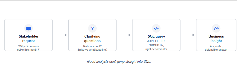
Read the stakeholder ask first and try to write your own query before looking at the solution. The clarifying questions matter as much as the SQL, since half of what separates a junior analyst from a senior one is knowing which assumption to check before running anything. If you haven't covered joins, window functions and CTEs yet, the SQL for Data Analysts guide is worth reading alongside this one, since several problems below assume that foundation rather than re-explaining it from scratch.

Every query here assumes fairly standard e-commerce or transactional table shapes, orders, customers, transactions, sessions, with obvious column names. Adjust table and column names to whatever schema you're actually working against; the pattern is the point, not the exact syntax. Examples use PostgreSQL-style syntax unless otherwise noted; problem 9 flags a dialect-specific keyword explicitly since it doesn't work the same way everywhere.

1. "Which products should we stop stocking?"

The business context: an e-commerce inventory manager wants to cut SKUs that are quietly costing money in storage and listing fees without asking directly for "slow-moving inventory," because that's not how the request usually arrives.

Clarifying questions to ask first: slow-moving compared to what benchmark? Over what time window? Should seasonal products be excluded, since a winter coat looking slow in July isn't the same signal as a year-round product looking slow in July?

The query:

sql

SELECT
    p.product_id,
    p.product_name,
    COUNT(o.order_id) AS orders_last_90_days,
    COALESCE(SUM(o.quantity), 0) AS units_sold_last_90_days
FROM products p
LEFT JOIN orders o
    ON p.product_id = o.product_id
    AND o.order_date >= CURRENT_DATE - INTERVAL '90 days'
GROUP BY p.product_id, p.product_name
HAVING COUNT(o.order_id) < 5
ORDER BY orders_last_90_days ASC;

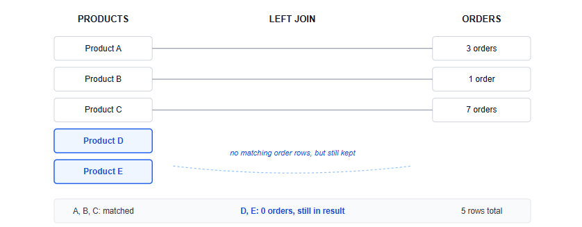
Why this approach: the LEFT JOIN is deliberate, not a default habit. An INNER JOIN would silently drop products with zero orders in the window, which are exactly the products this question is about. The date filter sits inside the JOIN condition rather than a WHERE clause, so products with no matching orders still appear in the result with a count of zero instead of disappearing entirely.

Common mistake: filtering with WHERE o.order_date >= ... instead of putting the condition in the JOIN. With a LEFT JOIN, a WHERE clause on the right-hand table silently converts it back into an INNER JOIN, because NULL rows fail the WHERE condition and get dropped.

2. "Why did the Bangalore market underperform this month?"

The business context: a food delivery operations lead has seen a dip in one city's numbers and wants to know if it's real or noise before escalating it.

Clarifying questions to ask first: underperform on what metric, orders, revenue, or average order value? Compared to last month, or the same month last year, given how much delivery demand shifts seasonally? Is "Bangalore" the full city or a specific set of delivery zones?

The query:

sql

SELECT
    city,
    DATE_TRUNC('month', order_date) AS order_month,
    COUNT(order_id) AS total_orders,
    SUM(order_value) AS total_revenue,
    ROUND(AVG(order_value), 2) AS avg_order_value
FROM orders
WHERE city = 'Bangalore'
    AND order_date >= CURRENT_DATE - INTERVAL '4 months'
GROUP BY city, DATE_TRUNC('month', order_date)
ORDER BY order_month;

Why this approach: pulling four months rather than two gives more context for judging whether the current change looks unusual relative to recent performance, rather than reacting to a single month in isolation. It isn't enough data to make a statistically rigorous claim about significance, just enough to see whether this month looks like a continuation of a trend or a genuine break from it. Breaking out order count, revenue and average order value separately matters, since a revenue dip with flat order count points to a different cause (lower basket size, a discount campaign) than a dip driven by order count alone (demand or supply issue).

Common mistake: stopping at total revenue without decomposing it into orders and average order value. A single blended number can't tell you whether fewer people ordered or the same people ordered less.

3. "How many users are stuck in a failed-payment loop?"

The business context: a fintech product manager suspects a payment gateway issue is causing users to retry and fail repeatedly, which quietly damages trust even if they eventually succeed.

Clarifying questions to ask first: how many failures in a row counts as "stuck," two, three, more? Within what time window, since a user retrying over three days is a different problem than one retrying in three minutes? Should eventual successes be excluded, or is the retry pattern itself the concern regardless of the outcome?

The query:

sql

WITH payment_attempts AS (
    SELECT
        user_id,
        transaction_id,
        status,
        attempted_at,
        ROW_NUMBER() OVER (
            PARTITION BY user_id ORDER BY attempted_at
        ) AS attempt_rank,
        ROW_NUMBER() OVER (
            PARTITION BY user_id, status ORDER BY attempted_at
        ) AS status_rank
    FROM transactions
    WHERE attempted_at >= CURRENT_DATE - INTERVAL '7 days'
),
failure_streaks AS (
    SELECT
        user_id,
        attempted_at,
        attempt_rank - status_rank AS streak_group
    FROM payment_attempts
    WHERE status = 'failed'
)
SELECT
    user_id,
    streak_group,
    COUNT(*) AS consecutive_failures,
    MIN(attempted_at) AS streak_started_at,
    MAX(attempted_at) AS streak_ended_at
FROM failure_streaks
GROUP BY user_id, streak_group
HAVING COUNT(*) >= 2
ORDER BY consecutive_failures DESC;

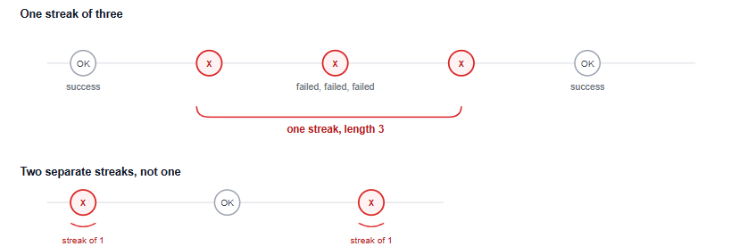
Why this approach: this is a gaps-and-islands problem, not a simple "compare to the row before" problem, and it's worth knowing the difference. attempt_rank numbers every attempt for a user in order, regardless of status; status_rank numbers only that user's failed attempts in order. While a run of failures has no successful attempt breaking it up, both ranks increase together, so attempt_rank - status_rank stays constant for the whole run and changes the moment a success interrupts it. Grouping on that difference correctly groups an unbroken run of failures into one streak, however long it is, rather than just flagging pairs.

A simpler LAG-based version, checking only whether the immediately previous attempt also failed, looks reasonable but produces the wrong answer here: three failures in a row would count as two separate matching rows instead of one streak of three, and it can't distinguish a single long streak from several short ones sitting next to each other. The gaps-and-islands version avoids both problems.

Common mistake: counting total failed transactions per user instead of consecutive ones. A user who failed once in January and once in June has nothing in common with a user who failed three times in ten minutes, but a plain COUNT treats them identically. The related mistake is reaching for LAG as if it solves streak-length counting on its own; it only tells you about the immediately adjacent row, not the full length of a run.

4. "Which customers are about to churn?"

The business context: a SaaS customer success lead wants a list of accounts showing early warning signs, not accounts that have already cancelled, since by then it's too late to intervene.

Clarifying questions to ask first: what does "about to churn" mean operationally, no login in X days, declining usage trend, or an approaching renewal date with low engagement? Does this need to cover all customers or just a specific plan tier?

The query:

sql

SELECT
    c.customer_id,
    c.company_name,
    MAX(l.login_date) AS last_login,
    CURRENT_DATE - MAX(l.login_date) AS days_since_last_login,
    CASE
        WHEN MAX(l.login_date) IS NULL THEN 'Never logged in'
        ELSE 'Previously logged in'
    END AS login_status,
    COUNT(l.login_date) FILTER (
        WHERE l.login_date >= CURRENT_DATE - INTERVAL '30 days'
    ) AS logins_last_30_days
FROM customers c
LEFT JOIN logins l ON c.customer_id = l.customer_id
WHERE c.subscription_status = 'active'
GROUP BY c.customer_id, c.company_name
HAVING MAX(l.login_date) < CURRENT_DATE - INTERVAL '14 days'
    OR MAX(l.login_date) IS NULL
ORDER BY days_since_last_login DESC NULLS FIRST;

Why this approach: the FILTER clause calculates a windowed count without needing a second CTE or subquery, which keeps the query readable for a fairly common reporting pattern. A customer who has never logged in has no rows at all in logins, so MAX(l.login_date) returns NULL for them, and days_since_last_login inherits that NULL rather than showing some default number, that's expected behaviour, not a bug. The login_status field makes that distinction explicit for whoever reads the output, rather than leaving them to interpret a blank cell. Ordering with NULLS FIRST deliberately surfaces customers who have never logged in at all, ahead of customers who logged in recently but stopped, since those tend to be the most urgent cases.

Common mistake: defining churn risk only by days since last login, without also looking at whether usage was trending down before it stopped. A customer who logged in daily until two weeks ago is a very different case from one who was already logging in once a month for the last quarter.

5. "What's driving the spike in returns?"

The business context: a D2C retail operations manager has seen the return rate jump and needs to know if it's one bad product, one bad region, or something broader before deciding what to fix.

Clarifying questions to ask first: spike relative to what baseline period? Return rate by order count or by revenue, since a handful of high-value returns can look different from many low-value ones? Can a single order generate more than one return record, for a multi-item order with a partial return, or is it safe to assume one return per order?

The query:

sql

SELECT
    p.category,
    COUNT(DISTINCT r.return_id) AS total_returns,
    COUNT(DISTINCT o.order_id) AS total_orders,
    ROUND(
        100.0 * COUNT(DISTINCT r.return_id) / NULLIF(COUNT(DISTINCT o.order_id), 0), 2
    ) AS return_rate_pct
FROM orders o
JOIN products p ON o.product_id = p.product_id
LEFT JOIN returns r ON o.order_id = r.order_id
WHERE o.order_date >= CURRENT_DATE - INTERVAL '60 days'
GROUP BY p.category
ORDER BY return_rate_pct DESC;

Why this approach: calculating a rate rather than a raw count of returns is the whole point of this query. Ten returns on a category with 50 orders is a serious problem; ten returns on a category with 5,000 orders is normal. The DISTINCT in both the numerator and denominator matters more than it looks: if a single order can generate more than one return record, a plain COUNT(o.order_id) on the joined result would count that order once for every matching return row, quietly inflating the order total along with the return total. Counting distinct order IDs and distinct return IDs keeps the two counts honest regardless of how many returns attach to one order. This still assumes one return record roughly corresponds to one return event; if a single return can itself span multiple rows, for instance, one row per returned line item, that's worth confirming with whoever owns the returns table before trusting the numerator. NULLIF guards against a division-by-zero error for any category with no orders in the window at all.

Common mistake: reporting the category with the most returns in absolute terms as "the problem," when it might just be the highest-volume category overall. The related, easier-to-miss mistake is joining orders to returns without DISTINCT and letting a handful of multi-return orders quietly inflate the order count, not just the return count, which understates the rate rather than overstating it.

6. "Are drivers being paid fairly relative to how much they're driving?"

The business context: a ride-hailing ops analyst has been asked to check whether payout is proportional to effort across drivers, ahead of a policy review.

Clarifying questions to ask first: "fairly" needs a defined comparison, pay per trip, pay per kilometre, or pay per hour online? Should cancelled or very short trips be excluded from the comparison?

The query:

sql

SELECT
    d.driver_id,
    COUNT(t.trip_id) AS total_trips,
    SUM(t.distance_km) AS total_distance_km,
    SUM(t.driver_payout) AS total_payout,
    ROUND(SUM(t.driver_payout) / NULLIF(SUM(t.distance_km), 0), 2) AS payout_per_km
FROM drivers d
JOIN trips t ON d.driver_id = t.driver_id
WHERE t.trip_status = 'completed'
    AND t.trip_date >= CURRENT_DATE - INTERVAL '30 days'
GROUP BY d.driver_id
ORDER BY payout_per_km ASC;

Why this approach: payout per kilometre is a normalised rate, which is what makes drivers with very different trip volumes actually comparable. Ordering ascending surfaces the drivers earning the least per kilometre first, which is where a deeper payout-equity review could start, not where it ends. Payout per kilometre doesn't by itself prove anything is unfair; trip type, time spent waiting for a rider to show up, surge or incentive payments, and traffic conditions can all legitimately shift this number without any actual unfairness in the underlying pay policy. Treat this as the metric that tells you where to look closer, not the metric that settles the question.

Common mistake: comparing total payout across drivers directly. A driver who completed 200 short trips will out-earn a driver who completed 50 long ones in total payout, without that meaning anything about fairness per unit of work. The mirror-image mistake is treating a low payout-per-kilometre driver as definitely underpaid without checking whether their trips involved more waiting time or worse traffic, both of which cost the driver time without adding distance.

7. "Show me the 90-day repeat purchase rate by first-purchase cohort."

The business context: an e-commerce growth lead wants to know whether more recent customer cohorts are stickier than older ones, to judge whether recent acquisition channels are bringing in better customers.

Clarifying questions to ask first: why 90 days specifically, does that match how often this business's customers would realistically reorder? Should one-time promotional or gift-card-only orders count toward "first purchase," or only genuine first-time customers?

The query:

sql

WITH first_orders AS (
    SELECT
        customer_id,
        MIN(order_date) AS first_order_date,
        DATE_TRUNC('month', MIN(order_date)) AS cohort_month
    FROM orders
    GROUP BY customer_id
),
mature_cohorts AS (
    SELECT customer_id, first_order_date, cohort_month
    FROM first_orders
    WHERE first_order_date <= CURRENT_DATE - INTERVAL '90 days'
),
repeat_flags AS (
    SELECT
        c.customer_id,
        c.cohort_month,
        EXISTS (
            SELECT 1
            FROM orders o
            WHERE o.customer_id = c.customer_id
                AND o.order_date > c.first_order_date
                AND o.order_date <= c.first_order_date + INTERVAL '90 days'
        ) AS repeated_within_90_days
    FROM mature_cohorts c
)
SELECT
    cohort_month,
    COUNT(*) AS cohort_size,
    COUNT(*) FILTER (WHERE repeated_within_90_days) AS repeat_customers,
    ROUND(
        100.0 * COUNT(*) FILTER (WHERE repeated_within_90_days) / COUNT(*), 2
    ) AS repeat_purchase_rate_90d_pct
FROM repeat_flags
GROUP BY cohort_month
ORDER BY cohort_month;

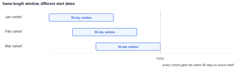
Why this approach: the cohort is defined by each customer's first order date because that's what the stakeholder actually asked for here, a first-purchase cohort, which keeps the analysis grounded in actual purchase behaviour rather than a separate signup event that may not exist in every business. The 90-day window is measured from each customer's own first order date, not from a shared calendar date, and mature_cohorts only includes customers whose 90-day window has already fully elapsed. That maturity filter is what actually makes the cohort comparison fair: without it, a cohort from last month would show an artificially low repeat rate purely because most of its customers haven't had 90 days to come back yet, not because they're genuinely less loyal than an older cohort. Equal observation windows are what make "is the March cohort stickier than the January cohort" a question this query can actually answer.

Common mistake: comparing repeat purchase rate across cohorts using "ever made a second order" instead of a fixed window. That approach systematically favours older cohorts, since they've simply had more calendar time to generate a second order, and can make a genuinely weaker recent cohort look fine just because it hasn't had time to prove otherwise yet.

8. "Which restaurants are losing customers after a bad review?"

The business context: a food delivery platform's quality team wants to know if there's a measurable customer drop-off after a restaurant's rating declines, to prioritise which partners need intervention.

Clarifying questions to ask first: how is "losing customers" measured, repeat order rate from existing customers, or overall order volume? What counts as a rating decline, a single bad review or a sustained drop in average rating?

The query:

sql

WITH monthly_ratings AS (
    SELECT
        restaurant_id,
        DATE_TRUNC('month', review_date) AS review_month,
        AVG(rating) AS avg_rating
    FROM reviews
    GROUP BY restaurant_id, DATE_TRUNC('month', review_date)
),
monthly_orders AS (
    SELECT
        restaurant_id,
        DATE_TRUNC('month', order_date) AS order_month,
        COUNT(DISTINCT customer_id) AS unique_customers
    FROM orders
    GROUP BY restaurant_id, DATE_TRUNC('month', order_date)
),
rating_changes AS (
    SELECT
        restaurant_id,
        review_month,
        avg_rating,
        avg_rating - LAG(avg_rating) OVER (
            PARTITION BY restaurant_id ORDER BY review_month
        ) AS rating_change
    FROM monthly_ratings
),
decline_months AS (
    SELECT restaurant_id, review_month AS decline_month
    FROM rating_changes
    WHERE rating_change <= -0.5
)
SELECT
    d.restaurant_id,
    d.decline_month,
    ROUND(AVG(o.unique_customers) FILTER (
        WHERE o.order_month BETWEEN d.decline_month - INTERVAL '3 months'
            AND d.decline_month - INTERVAL '1 month'
    ), 1) AS avg_customers_before,
    ROUND(AVG(o.unique_customers) FILTER (
        WHERE o.order_month BETWEEN d.decline_month + INTERVAL '1 month'
            AND d.decline_month + INTERVAL '3 months'
    ), 1) AS avg_customers_after
FROM decline_months d
JOIN monthly_orders o ON d.restaurant_id = o.restaurant_id
GROUP BY d.restaurant_id, d.decline_month
ORDER BY d.restaurant_id, d.decline_month;

Why this approach: a side-by-side trend of rating and customer counts leaves the reader to eyeball a connection, which isn't the same as actually answering "are restaurants with declining ratings also seeing customer declines." This version answers it directly: rating_changes uses LAG to detect a genuine month-over-month drop of at least half a star, then the final query compares each restaurant's average monthly customers in the three months before that decline against the three months after. That's a real before/after comparison, not a side-by-side trend the reader has to interpret unaided.

Worth being precise about what the AVG in the final query is actually averaging over: monthly_orders only contains a row for a restaurant-month if that restaurant had at least one order that month, so a restaurant with a genuinely dead month, zero orders, simply has no row for it rather than a row showing zero. The before/after averages here are averages of the months that had any recorded activity, not a strict three-month average with dead months counted as zero. For most restaurants with reasonably steady volume this distinction won't change the picture, but for a restaurant with a very sparse order history, it's worth checking how many months actually contributed to each average before treating the comparison as solid.

This still isn't proof of causation, and the query doesn't claim otherwise. A restaurant could see falling customers and a falling rating at the same time for a shared third reason, a change in delivery times, a new competitor, a menu change, rather than one causing the other. What this query adds is a specific, comparable before/after number an analyst can point to when deciding which restaurants are worth investigating further, rather than a vague impression from eyeballing two separate lines on a chart.

Common mistake: treating a correlation found in this output as proof the rating drop caused the customer drop. A cuisine going out of seasonal favour, a nearby competitor opening, or a delivery-time issue could produce the same pattern. This query surfaces the pattern; explaining it is a separate step. The quieter mistake is assuming the before/after average always covers exactly three full months per restaurant; a restaurant with sparse order history may have fewer contributing months than that, which is worth a sanity check before drawing a conclusion.

9. "Are we getting charged twice for the same transaction?"

The business context: a fintech finance team suspects a reconciliation issue is producing duplicate charges and needs them identified before the next settlement cycle.

Clarifying questions to ask first: what counts as a duplicate, an exact match on amount, customer and timestamp, or a near-match within a short time window, since retries with slightly different timestamps are a common real-world pattern? Should genuinely repeated legitimate charges, like two separate coffee purchases, be excluded?

The query:

sql

SELECT
    customer_id,
    amount,
    transaction_id,
    created_at,
    COUNT(*) OVER (
        PARTITION BY customer_id, amount,
        DATE_TRUNC('minute', created_at)
    ) AS matches_in_same_minute
FROM transactions
WHERE created_at >= CURRENT_DATE - INTERVAL '7 days'
QUALIFY matches_in_same_minute > 1
ORDER BY customer_id, created_at;

Note: QUALIFY is supported in Snowflake, BigQuery and DuckDB but not in PostgreSQL or MySQL; in those, wrap the window function in a CTE and filter with an outer WHERE clause instead.

Why this approach: partitioning by customer, amount and the same minute, rather than requiring an exact timestamp match, catches the realistic case of a retry landing a few seconds apart, which an exact-match approach would miss entirely. These are candidate duplicate charges for investigation, not confirmed duplicate transactions. Legitimate repeated purchases can still match this pattern, so the output is a shortlist worth checking, not a finished fraud or billing-error report.

Common mistake: matching only on transaction amount across the whole table, without partitioning by customer and time. Two unrelated customers buying the same ₹499 subscription in the same week will match on amount alone and generate false positives.

10. "What's our month-over-month revenue growth?"

The business context: a SaaS finance lead needs a clean growth trend for a board update, not just a table of monthly totals that requires manual comparison.

Clarifying questions to ask first: growth in new revenue, total revenue, or net revenue after cancellations? Should the most recent partial month be included, since an in-progress month will always look like a decline compared to a completed one?

The query:

sql

WITH monthly_revenue AS (
    SELECT
        DATE_TRUNC('month', payment_date) AS revenue_month,
        SUM(amount) AS total_revenue
    FROM payments
    WHERE payment_date < DATE_TRUNC('month', CURRENT_DATE)
    GROUP BY DATE_TRUNC('month', payment_date)
)
SELECT
    revenue_month,
    total_revenue,
    LAG(total_revenue) OVER (ORDER BY revenue_month) AS prior_month_revenue,
    ROUND(
        100.0 * (total_revenue - LAG(total_revenue) OVER (ORDER BY revenue_month))
        / NULLIF(LAG(total_revenue) OVER (ORDER BY revenue_month), 0), 2
    ) AS mom_growth_pct
FROM monthly_revenue
ORDER BY revenue_month;

Why this approach: excluding the current, still-in-progress month in the WHERE clause avoids the most common way this exact report misleads a stakeholder. LAG pulls the prior month into the same row so the growth percentage can be calculated directly, without a self-join.

Common mistake: including the current partial month in a month-over-month comparison. Every month will appear to be declining right up until it closes, which routinely triggers false alarm in exactly this kind of report.

11. "Which marketing channel actually brings in the best customers, not just the most signups?"

The business context: a D2C growth lead wants to shift budget toward channels that bring in customers who spend more over time, not just the channel with the lowest cost per signup.

Clarifying questions to ask first: "best" needs a definition, total revenue per customer, order frequency, or both? What's a fair comparison window after acquisition, since a customer who signed up yesterday hasn't had the same chance to spend as one who signed up six months ago, and comparing them on total revenue to date would unfairly favour whichever channel happened to bring in older customers?

The query:

sql

SELECT
    c.acquisition_channel,
    COUNT(DISTINCT c.customer_id) AS customers_acquired,
    SUM(o.order_value) AS revenue_within_90_days,
    ROUND(
        SUM(o.order_value) / COUNT(DISTINCT c.customer_id), 2
    ) AS revenue_per_customer_90d
FROM customers c
LEFT JOIN orders o
    ON c.customer_id = o.customer_id
    AND o.order_date BETWEEN c.signup_date AND c.signup_date + INTERVAL '90 days'
WHERE c.signup_date <= CURRENT_DATE - INTERVAL '90 days'
GROUP BY c.acquisition_channel
ORDER BY revenue_per_customer_90d DESC;

Why this approach: this compares every customer over the same fixed 90-day window measured from their own signup date, not from a shared calendar date, which is what makes the comparison fair. The WHERE clause only includes customers who signed up at least 90 days ago, so every customer counted has actually had the full window to generate revenue; a customer who signed up last week is excluded entirely rather than counted with an artificially low, still-accumulating total. LEFT JOIN matters here too: a customer acquired through a channel who never ordered anything is still real information about that channel's quality, and an INNER JOIN would silently drop them from both the numerator and the denominator instead of counting them as a zero.

Common mistake: ranking channels by total revenue rather than revenue per customer, which systematically favours high-volume channels over high-quality ones and can send budget in exactly the wrong direction. The subtler version of this mistake is comparing revenue per customer across a mix of old and recently acquired customers without a fixed post-acquisition window; that quietly favours whichever channel happened to bring in older customers, regardless of which channel's customers actually spend more, faster.

12. "What's our busiest hour, by city?"

The business context: a ride-hailing operations team is planning driver incentive shifts and needs to know when demand actually peaks in each city, since assuming it's the same everywhere usually isn't true.

Clarifying questions to ask first: busiest by trip count or by revenue, since a lunchtime peak in trip count doesn't always match an evening peak in fare value? Should weekends be analysed separately from weekdays?

The query:

sql

SELECT
    city,
    EXTRACT(HOUR FROM requested_at) AS hour_of_day,
    COUNT(trip_id) AS total_trips
FROM trips
WHERE requested_at >= CURRENT_DATE - INTERVAL '30 days'
    AND EXTRACT(DOW FROM requested_at) BETWEEN 1 AND 5
GROUP BY city, EXTRACT(HOUR FROM requested_at)
ORDER BY city, total_trips DESC;

Why this approach: filtering to weekdays only keeps this specific version of the answer focused on a single, consistent pattern rather than blending two different demand curves into one misleading average. In PostgreSQL, EXTRACT(DOW FROM ...) returns 0 for Sunday through 6 for Saturday, so BETWEEN 1 AND 5 correctly captures Monday through Friday; other dialects number the days differently (MySQL's DAYOFWEEK, for example, returns 1 for Sunday), so double-check this against whichever engine you're actually running against before reusing it.

Common mistake: averaging weekday and weekend demand together. A city with a sharp weekday commute peak and flat weekend demand will show a blended pattern that doesn't actually describe either day type accurately.

13. "Which customers used to order frequently but have gone quiet?"

The business context: an e-commerce retention team wants a list of lapsed high-value customers to target with a win-back campaign, specifically excluding customers who were never frequent buyers in the first place.

Clarifying questions to ask first: how is "used to order frequently" defined, a minimum number of orders in a prior period? How long counts as "gone quiet," 60 days, 90 days?

The query:

sql

WITH customer_history AS (
    SELECT
        customer_id,
        COUNT(order_id) FILTER (
            WHERE order_date BETWEEN CURRENT_DATE - INTERVAL '180 days'
                AND CURRENT_DATE - INTERVAL '60 days'
        ) AS orders_prior_period,
        MAX(order_date) AS last_order_date
    FROM orders
    GROUP BY customer_id
)
SELECT
    customer_id,
    orders_prior_period,
    last_order_date,
    CURRENT_DATE - last_order_date AS days_since_last_order
FROM customer_history
WHERE orders_prior_period >= 3
    AND last_order_date < CURRENT_DATE - INTERVAL '60 days'
ORDER BY orders_prior_period DESC;

Why this approach: splitting the timeline into a "prior period" for establishing frequency and a separate "recent" cutoff for lapsing keeps the two conditions independently adjustable. This specifically excludes customers who simply never ordered much, which a single "no orders in 60 days" filter would incorrectly sweep in alongside genuinely valuable lapsed customers.

Common mistake: defining "gone quiet" using only a recency filter, without a frequency filter first. That approach flags every low-value, rarely-purchasing customer alongside the genuinely valuable ones a win-back campaign should actually prioritise.

14. "Where are we losing users between KYC and their first transaction?"

The business context: a fintech product team suspects the onboarding funnel is leaking users somewhere between identity verification and actually using the product, and needs to know which step.

Clarifying questions to ask first: what are the exact funnel steps in order, since "KYC" might itself be multiple stages (document upload, verification, approval)? What counts as a completed step, a status flag, a timestamp, or both?

The query:

sql

WITH funnel_counts AS (
    SELECT
        COUNT(DISTINCT user_id) AS total_users,
        COUNT(DISTINCT user_id) FILTER (WHERE kyc_started_at IS NOT NULL) AS kyc_started,
        COUNT(DISTINCT user_id) FILTER (WHERE kyc_completed_at IS NOT NULL) AS kyc_completed,
        COUNT(DISTINCT user_id) FILTER (WHERE first_transaction_at IS NOT NULL) AS made_first_transaction
    FROM user_funnel
    WHERE signup_date >= CURRENT_DATE - INTERVAL '90 days'
)
SELECT
    total_users,
    kyc_started,
    ROUND(100.0 * kyc_started / NULLIF(total_users, 0), 1) AS kyc_started_pct_of_total,
    kyc_completed,
    ROUND(100.0 * kyc_completed / NULLIF(total_users, 0), 1) AS kyc_completed_pct_of_total,
    ROUND(100.0 * kyc_completed / NULLIF(kyc_started, 0), 1) AS kyc_completed_pct_of_prior_step,
    made_first_transaction,
    ROUND(100.0 * made_first_transaction / NULLIF(total_users, 0), 1) AS first_transaction_pct_of_total,
    ROUND(100.0 * made_first_transaction / NULLIF(kyc_completed, 0), 1) AS first_transaction_pct_of_prior_step
FROM funnel_counts;

Why this approach: using FILTER against a single pre-joined funnel table produces all four stage counts in one pass, which is both simpler and faster than four separate queries. The outer query then calculates each stage two ways, as a percentage of the original signup total and as a percentage of the immediately prior step, because those two numbers can tell very different stories. A step might look fine against the stage right before it while still representing a large cumulative loss from the very first stage; showing both numbers side by side, rather than making the reader infer one from the other, is what actually prevents that from being missed.

Common mistake: calculating each funnel stage as a percentage of the previous stage only, without also showing the percentage of the original total. A 90% completion rate from step three to step four sounds fine in isolation, but hides a much larger cumulative loss from step one if the earlier drop-off was already severe.

15. "Are free trial users converting to paid, and how long does it take them?"

The business context: a SaaS product lead wants to know both the conversion rate and the typical time-to-convert, since a healthy conversion rate that takes four months to materialise has very different implications than one that happens in the first week.

Clarifying questions to ask first: should trials that are still in progress be included or excluded from the conversion rate calculation? Is "converting" the first payment, or does it need to survive past a refund window?

The query:

sql

WITH trial_outcomes AS (
    SELECT
        user_id,
        trial_start_date,
        first_payment_date,
        first_payment_date IS NOT NULL AS converted,
        first_payment_date - trial_start_date AS days_to_convert
    FROM trial_users
    WHERE trial_start_date <= CURRENT_DATE - INTERVAL '30 days'
)
SELECT
    COUNT(*) AS total_trials,
    COUNT(*) FILTER (WHERE converted) AS total_conversions,
    ROUND(
        100.0 * COUNT(*) FILTER (WHERE converted) / NULLIF(COUNT(*), 0), 2
    ) AS conversion_rate_pct,
    ROUND(AVG(days_to_convert) FILTER (WHERE converted), 1) AS avg_days_to_convert
FROM trial_outcomes;

Why this approach: filtering to trials that started at least 30 days ago avoids counting a still-open, unconverted trial as a failure before it's had a fair chance to convert, which would understate the real conversion rate.

Common mistake: calculating the conversion rate across all trials regardless of how recently they started. Trials that began yesterday haven't had time to convert yet, and including them makes a perfectly healthy conversion rate look artificially low.

Common mistakes across all fifteen problems

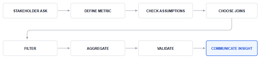
• Writing the query before asking what the stakeholder actually means. Half the problems above hinge on a definition, "underperform," "fairly," "gone quiet," that has more than one reasonable interpretation. Asking first is faster than writing three wrong versions.

• Reporting a count when a rate was the actual question. Returns, churn and conversion all showed up in this list specifically because raw counts mislead in each case without a denominator to compare against.

• Filtering inside WHERE when the logic belongs in the JOIN, or vice versa. Getting this backwards with an outer join is one of the most common ways a query silently returns the wrong answer without erroring.

• Treating a correlation the query surfaces as an explanation. Several of these queries, especially the rating and return-rate problems, produce a pattern worth investigating, not a proven cause. Say so explicitly when handing off the result.

Where to go from here

These fifteen problems assume comfort with joins, GROUP BY, window functions and CTEs already in place. If any of the syntax here felt unfamiliar rather than just the business framing, it's worth circling back to those fundamentals first, and the Top 100 SQL Interview Questions resource is a good next stop for interview-specific practice once these feel comfortable. Several of these fifteen problems are close cousins of the case-study questions covered in the interview questions guide, since a stakeholder-style SQL problem is exactly what shows up in a live technical round.

The cohort and funnel-style problems in this set, numbers 7, 13 and 14 especially, connect directly to product analytics; the statistics guide is worth reading next if you want to go a step further and reason about whether a pattern like the review-to-orders correlation in problem 8 is actually significant, not just visible.