Why Every Programmer Needs to Know Arrays ?

Imagine you're building a scoreboard for an online game. You have 1,000 players, each with a score. Would you create 1,000 separate variables  score1, score2, score3 ... score1000? Of course not. You'd use an array.

Arrays are the backbone of nearly every program ever written. Whether you're building a social media app, a machine learning model, a game engine, or a simple calculator arrays are there, quietly doing the heavy lifting.

Yet many beginners rush past them to learn "cooler" things like recursion or object-oriented programming, only to come back later and realise they didn't fully understand the foundation.

This guide fixes that. We'll go from the very basics all the way to how arrays work at the hardware level, algorithm patterns built on top of them, and the mistakes even experienced developers make.

What is an Array?

An array is a collection of elements stored at contiguous (adjacent) memory locations, where each element is of the same data type and can be accessed directly by its position (called an index).

Break that definition apart:

• Collection of elements — it stores multiple values, not just one

• Contiguous memory — all values sit next to each other in RAM, no gaps

• Same data type — (in strict languages) all items are integers, or all strings, etc.

• Direct access via index — you can jump to any element instantly

Key Analogy:

Think of an array like a row of numbered lockers. Each locker has a unique number (the index), and you can open any locker directly without opening all the ones before it.

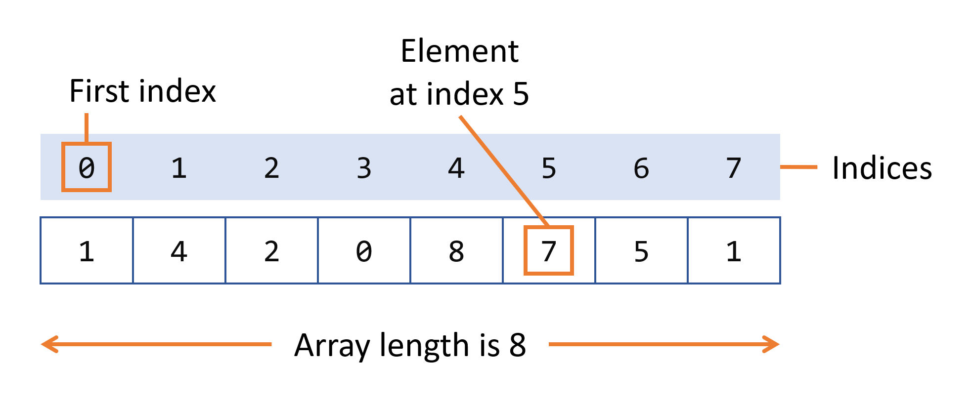
Let's say we create an array called myFruits having three values:

'banana'- index 0

'apple' - index 1

'orange' - index 2

Notice that the first element is at index 0, not 1. This is called zero-based indexing and is the standard in most programming languages. We'll explain exactly why this is the case in the Indexing section.

Creating an Array

Here's how you create the myFruits array in different languages:

// JavaScript — flexible, can hold mixed types
const myFruits = ['banana', 'apple', 'orange'];
console.log(myFruits);  // ['banana', 'apple', 'orange']

How Arrays Work in Memory

This is the section most beginner tutorials skip, but it's the key to understanding why arrays behave the way they do.

When your program runs, it uses RAM (Random Access Memory) to store data. Think of RAM as a very long street of numbered houses. Each house has a unique address and holds exactly one byte of data.

When you create an array, the computer reserves a contiguous block of these memory addresses, like booking a row of adjacent houses on this street. No gaps, no skipping. All the values sit right next to each other.

Why Does Contiguous Memory Matter for Performance?

Modern CPUs have a cache a small, ultra-fast memory chip. When you access an array element, the CPU often loads a chunk of nearby memory addresses into cache automatically.

Because array elements sit next to each other, reading the next element is almost instant, it's already in cache. This is called cache locality and is one reason arrays can outperform other data structures in practice.

Cache Locality: Arrays benefit from CPU cache prefetching. When you access arr[0], the CPU loads arr[1], arr[2], arr[3] into cache too making subsequent accesses nearly instant.

Types of Arrays

Based on Dimensions:

• 1 D Array: A simple linear list. Each element is accessed with a single index. Best for lists, sequences, and simple collections.

• 2D Array: A grid of rows and columns (matrix). Access with two indices [row][col]. Used for tables, spreadsheets, and game boards.

• 3D Array: Adds a "depth" dimension. Three indices required. Used in 3D graphics, volumetric data, and simulations.

• N-Dimensional: Arrays of any number of dimensions. Common in scientific computing with libraries like NumPy for tensor operations.

Based on Size

Fixed-Size Arrays

In languages like C, C++, and Java, when you declare an array you must specify its size upfront. That size is locked, you can't add an 11th element to an array of 10.

// Fixed-size array in Java — size is 5, cannot change
int[] scores = new int[5];
scores[0] = 85;
scores[1] = 92;
// scores[5] = 78;  ← This would throw ArrayIndexOutOfBoundsException!

Dynamic Arrays

Dynamic arrays can grow and shrink at runtime. Python's list and JavaScript's Array are dynamic by default. Under the hood, when a dynamic array runs out of space, it allocates a larger block and copies all existing elements over.

Specialised Array Types

• Jagged Array: An array of arrays where inner arrays can have different lengths. Memory efficient for uneven data sets (e.g., a triangle-shaped grid).

• Sparse Array: Most values are zero or empty. Only non-zero values and their indices are stored. Essential for large scientific datasets.

• Associative Array: Uses string keys instead of numeric indexes. Python's dict, JavaScript Object, and Java's HashMap are examples.

• Circular Array: The last element wraps around to connect to the first. Used in queues and buffering systems (e.g., audio/video buffers).

Array Indexing Explained

Why Does Indexing Start at 0?

This confuses almost every beginner. If an array has 3 elements, why are they at positions 0, 1, and 2, not 1, 2, and 3?

Remember the address formula: Address = Base + (index × size). If indexing started at 1, the formula would be Base + ((index - 1) × size) an extra subtraction on every single array access. Zero-based indexing makes the math cleaner and faster.

• Zero-based indexing is used by: C, C++, Java, Python, JavaScript, Go, Rust, Swift.

• One-based indexing is used by: MATLAB, Lua, R, Fortran.

Negative Indexing (Python)

Python supports negative indexing, which counts from the end of the array. arr[-1] gives the last element, arr[-2] gives the second-to-last, and so on.

fruits = ['banana', 'apple', 'orange', 'kiwi']

Core Array Operations

Time Complexity Overview

1. Reading / Accessing Elements

Access any element in O(1) time using its index. This is the array's biggest strength.

fruits = ['banana', 'apple', 'orange']

print(fruits[0])   # banana  (first element)
print(fruits[2])   # orange  (last element)
print(fruits[-1])  # orange  (Python negative index)

2. Updating Elements

Replace the value at an index using the assignment operator. Also O(1).

fruits = ['banana', 'apple', 'orange']
fruits[0] = 'kiwi'   # Replace 'banana' with 'kiwi'
print(fruits)  # ['kiwi', 'apple', 'orange']

3. Inserting Elements

Inserting at the end is fast (O(1)). Inserting in the middle or beginning requires shifting all subsequent elements O(n).

fruits = ['banana', 'apple', 'orange']

# Insert at the END — O(1) amortized
fruits.append('kiwi')
# ['banana', 'apple', 'orange', 'kiwi']

# Insert at a specific index — O(n)
fruits.insert(1, 'mango')
# ['banana', 'mango', 'apple', 'orange', 'kiwi']

4. Deleting Elements

fruits = ['banana', 'apple', 'orange', 'kiwi']

# Remove by index
fruits.pop(1)       # removes 'apple'
# ['banana', 'orange', 'kiwi']

# Remove by value
fruits.remove('kiwi')  # removes first occurrence of 'kiwi'
# ['banana', 'orange']

5. Searching an Array

There are two main searching approaches depending on whether the array is sorted.

Linear Search — O(n)

Check every element one by one until you find the target. Works on any array, sorted or not.

def linear_search(arr, target):
    for i in range(len(arr)):
        if arr[i] == target:
            return i   # Return index if found
    return -1           # Return -1 if not found

names = ['Alice', 'Bob', 'Charlie', 'Diana']
print(linear_search(names, 'Charlie'))  # Output: 2

Binary Search — O(log n)

Only works on sorted arrays. Cuts the search space in half with each comparison, dramatically faster for large arrays.

def binary_search(arr, target):
    left, right = 0, len(arr) - 1
    while left <= right:
        mid = (left + right) // 2
        if arr[mid] == target:
            return mid              # Found!
        elif arr[mid] < target:
            left = mid + 1          # Search right half
        else:
            right = mid - 1         # Search left half
    return -1

sorted_nums = [2, 5, 8, 12, 16, 23, 38, 56]
print(binary_search(sorted_nums, 23))  # Output: 5

6. Traversal — Looping Through an Array

scores = [85, 92, 78, 95, 88]

# Method 1: for-each (most Pythonic)
for score in scores:
    print(score)

# Method 2: index-based loop
for i in range(len(scores)):
    print(f"Index {i}: {scores[i]}")

# Method 3: enumerate (index + value)
for i, score in enumerate(scores):
    print(f"Player {i+1} scored: {score}")

Multi-Dimensional Arrays In Depth

A 2D array is an array of arrays a grid with rows and columns. You need two indexes to access any element: one for the row and one for the column.

Creating and Using a 2D Array

# Creating a 3x3 matrix
matrix = [
    [1, 2, 3],
    [4, 5, 6],
    [7, 8, 9]
]

# Access element at row 1, column 2
print(matrix[1][2])  # Output: 6

# Traverse all elements
for row in matrix:
    for val in row:
        print(val, end=" ")
    print()

Arrays vs Other Data Structures

When to Use Arrays vs When Not To

✅ Use Arrays When

• You need fast random access by index

• The data is sequential and ordered

• The collection size is known or roughly bounded

• Working with mathematical data (matrices, vectors)

• Cache performance matters (loops over large data)

• Implementing other data structures (stack, queue)

❌ Avoid Arrays When

• Frequent insertions/deletions in the middle

• Data size varies dramatically and unpredictably

• You need to frequently search by value (use HashMap)

• Data has natural key-value pairing (use dict/map)

• Hierarchical data (use trees)

Arrays Across Programming Languages

Real-World Use Cases of Arrays

Arrays aren't just a textbook concept. They're baked into the fabric of real software.

1. Game Scoreboards: All player scores stored in one array. Sort it in one line to get a leaderboard instantly.

2. Image Processing: A JPEG image is just a 2D (or 3D for RGB) array of pixel values. Every filter and effect manipulates this array.

3. Undo/Redo History: Text editors store a history of states in an array. Ctrl+Z pops the last state from the end.

4. Audio Streaming: Sound is stored as arrays of amplitude values. Circular arrays serve as ring buffers for real-time audio.

5. Spreadsheets; Every spreadsheet (Excel, Google Sheets) is a 2D array under the hood — rows and columns of cell values.

6. Machine Learning: Neural network weights, training datasets, and model inputs/outputs are all multidimensional arrays (tensors).

7. Web Development: API responses return JSON arrays. React renders lists from arrays. DOM manipulation uses array-like NodeLists.

8. Stock Price Charts: Time-series stock data is an array of prices. Chart libraries like D3.js simply loop over an array to draw graphs.

Advanced Array Concepts

How Dynamic Arrays Grow (Amortized O(1))

When Python's list runs out of space, it doesn't just add one slot. It allocates roughly double the current capacity, copies all elements, and discards the old block.

This means most appends are instant, but occasional ones trigger a resize. Averaged over many operations, the cost per append is still O(1), this is called amortized constant time.

Growth Factor: Python uses a growth factor of ~1.125x, JavaScript engines typically use 2x. Java's ArrayList uses 1.5x. The exact factor is a tradeoff between wasted memory (too large) and frequency of copying (too small).

The Sliding Window Technique

One of the most powerful array algorithm patterns. Instead of recomputing a subarray sum from scratch each time, you slide a "window" across the array, adding the new element and removing the old one in O(1).

# Find the maximum sum of any 3 consecutive elements
def max_window_sum(arr, k):
    window_sum = sum(arr[:k])   # sum of first window
    max_sum = window_sum

    for i in range(k, len(arr)):
        # Slide: add new element, remove oldest
        window_sum += arr[i] - arr[i - k]
        max_sum = max(max_sum, window_sum)

    return max_sum

print(max_window_sum([2, 1, 5, 1, 3, 2], 3))  # Output: 9  (5+1+3)

The Two-Pointer Technique

Use two pointers that start at opposite ends of a sorted array and move toward each other. Efficient for problems like finding pairs that sum to a target.

# Check if two elements in a sorted array sum to target
def two_sum_sorted(arr, target):
    left, right = 0, len(arr) - 1
    while left < right:
        current = arr[left] + arr[right]
        if current == target:
            return (left, right)
        elif current < target:
            left += 1   # Need bigger sum — move left pointer right
        else:
            right -= 1  # Need smaller sum — move right pointer left
    return None

print(two_sum_sorted([1, 3, 5, 7, 9], 12))  # Output: (2, 4) → arr[2]+arr[4]=5+9=14? No → (1,4)→3+9=12 ✓

Conclusion

Arrays are deceptively simple on the surface but surprisingly deep once you understand how they work in memory. Let's recap what we covered:

• An array is a collection of values stored in contiguous memory, accessible in O(1) by index.

• Arrays can be 1D, 2D, 3D, fixed-size, or dynamic depending on language and use case.

• Reading is O(1). Searching, inserting in the middle, and deleting are O(n).

• Contiguous memory gives arrays excellent cache locality, a real-world performance advantage.

• Different languages implement arrays differently, but the underlying concept is universal.

• Common algorithms like binary search, sliding window, and two-pointer are all built on top of arrays.

​

Arrays are the foundation upon which stacks, queues, hash tables, heaps, and many other data structures are built. A deep understanding of arrays is the first and most important, step on your data structures and algorithms journey.