SQL Window Functions Explained: 10 Real-World Examples for Data Analysts

SQL Window Functions Explained: 10 Real-World Examples for Data Analysts

Window functions are the feature that separates a query that filters and aggregates from a query that actually answers an analytical question. GROUP BY collapses rows. A window function calculates across a set of related rows while keeping every row in the output, which is what lets you compute a running total, a rank, or a period-over-period comparison without a self-join or a subquery.

If you have ever written a self-join to compare a row to the row before it, a window function replaces that pattern in one line. This article covers the syntax once, then works through ten patterns you will hit repeatedly as a data analyst: running totals, rankings, period comparisons, moving averages, and deduplication.

How Window Functions Are Structured

Every window function has the same three parts: the function itself, an optional PARTITION BY that defines the groups to calculate within, and an ORDER BY that defines the sequence the function operates over. Some functions also take a frame clause that narrows the window to a specific range of rows around the current one.

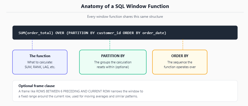
Anatomy of a SQL window function showing the function, PARTITION BY, ORDER BY, and optional frame clause labeled on a real query

-- Anatomy: function() OVER (PARTITION BY ... ORDER BY ... [frame])
SELECT
    order_id,
    customer_id,
    order_date,
    order_total,
    SUM(order_total) OVER (
        PARTITION BY customer_id
        ORDER BY order_date
    ) AS running_customer_total
FROM orders;

Everything below builds on this shape. The PostgreSQL window functions documentation is the most complete reference for the full list of available functions and frame syntax if you need something beyond the ten patterns here.

Window Functions vs. GROUP BY

The reason window functions matter for analysts specifically is that they do not collapse the result set. A GROUP BY query answers “what is the total per customer,” one row per customer. A window function can answer the same aggregate question while still showing every order row, which is what you need for a report that shows both the individual transaction and its running context.

This is why a query asking “show me each order and what percentage it represents of that customer’s total spend” needs a window function. A GROUP BY alone cannot return the order-level detail and the group-level percentage in the same row without a self-join back to the aggregated result.

The Ten Patterns

1. Running Total

A running total (cumulative sum) answers “what has accumulated up to this row.” The default frame for ORDER BY without an explicit frame clause is everything from the start of the partition up to the current row, which is exactly what a running total needs.

SELECT
    order_date,
    daily_revenue,
    SUM(daily_revenue) OVER (ORDER BY order_date) AS cumulative_revenue
FROM daily_revenue_summary;

2. Ranking Within a Group

RANK() assigns a position within each partition, restarting at 1 for every group. This is the pattern behind “top 3 products per category” style questions.

SELECT
    category,
    product_name,
    units_sold,
    RANK() OVER (PARTITION BY category ORDER BY units_sold DESC) AS rank_in_category
FROM product_sales;

3. Comparing a Row to the Previous One (LAG)

LAG() pulls a value from a prior row in the same ordered partition, which removes the need for a self-join when comparing a metric period over period.

SELECT
    month,
    monthly_active_users,
    LAG(monthly_active_users) OVER (ORDER BY month) AS previous_month_mau,
    monthly_active_users - LAG(monthly_active_users) OVER (ORDER BY month) AS mau_change
FROM monthly_metrics;

4. Comparing a Row to the Next One (LEAD)

LEAD() is the mirror of LAG(), useful for questions like “how many days until this customer’s next order,” which is a common building block in retention and cadence analysis.

SELECT
    customer_id,
    order_date,
    LEAD(order_date) OVER (PARTITION BY customer_id ORDER BY order_date) AS next_order_date,
    LEAD(order_date) OVER (PARTITION BY customer_id ORDER BY order_date) - order_date AS days_to_next_order
FROM orders;

Note that date subtraction syntax here returns an interval in PostgreSQL; other engines may require a function like DATEDIFF() instead, so check your engine’s date-handling documentation, such as MySQL’s documentation, before reusing this exact line.

5. Moving Average

A frame clause restricts the window to a fixed number of rows around the current one, which is how a trailing moving average is built.

SELECT
    order_date,
    daily_revenue,
    AVG(daily_revenue) OVER (
        ORDER BY order_date
        ROWS BETWEEN 6 PRECEDING AND CURRENT ROW
    ) AS trailing_7_day_avg
FROM daily_revenue_summary;

6. Percent of Group Total

Dividing a row’s value by the partition’s total, computed with the same window function pattern, gives a percent-of-total without a separate aggregation subquery.

SELECT
    region,
    salesperson,
    sales_amount,
    ROUND(
        100.0 * sales_amount / SUM(sales_amount) OVER (PARTITION BY region),
        1
    ) AS pct_of_region_sales
FROM sales;

7. First and Last Value in a Partition

FIRST_VALUE() and LAST_VALUE() return a value from the edge of the window, useful for questions like “what was each customer’s first purchase amount,” which otherwise requires a correlated subquery.

SELECT DISTINCT
    customer_id,
    FIRST_VALUE(order_total) OVER (
        PARTITION BY customer_id ORDER BY order_date
    ) AS first_order_total
FROM orders;

LAST_VALUE() requires an explicit frame extending to the end of the partition (ROWS BETWEEN CURRENT ROW AND UNBOUNDED FOLLOWING) in most engines, since the default frame only looks backward from the current row. Skipping that frame clause is a common source of a LAST_VALUE() query silently returning the current row’s own value instead of the true last row.

8. Deduplication with ROW_NUMBER

ROW_NUMBER() assigns a strictly increasing number within a partition, even when values tie, which makes it the standard tool for keeping only the most recent record per key.

SELECT *
FROM (
    SELECT
        *,
        ROW_NUMBER() OVER (
            PARTITION BY customer_id ORDER BY updated_at DESC
        ) AS row_num
    FROM customer_records
) ranked
WHERE row_num = 1;

This pattern is one of the most common fixes for a source table that has accumulated duplicate or superseded rows per key, a scenario also covered from the cleanup side in the Gradient Learnings guide to cleaning messy data in Excel for cases where the deduplication has to happen before the data ever reaches SQL.

9. Segmenting Rows into Buckets with NTILE

NTILE(n) splits a partition into n roughly equal-sized groups, ordered by the specified column, which is a quick way to build quartiles or quintiles for a metric like customer lifetime value.

SELECT
    customer_id,
    lifetime_value,
    NTILE(4) OVER (ORDER BY lifetime_value DESC) AS value_quartile
FROM customer_summary;

10. Handling Ties: RANK vs. DENSE_RANK

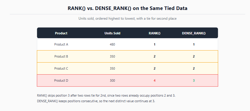
RANK() and DENSE_RANK() both handle ties, but they diverge in what happens after one: RANK() skips the next position(s) equal to the number of tied rows, while DENSE_RANK() does not skip any position.

SELECT
    product_name,
    units_sold,
    RANK() OVER (ORDER BY units_sold DESC) AS rank_with_gaps,
    DENSE_RANK() OVER (ORDER BY units_sold DESC) AS rank_no_gaps
FROM product_sales;

If two products tie for 2nd place, RANK() places the next distinct product at 4th, while DENSE_RANK() places it at 3rd. Which one is correct depends entirely on what the ranking is meant to represent, for example a leaderboard where skipped positions matter versus a tier assignment where they do not.

​

Common Mistakes / Practical Checklist

• Forgetting PARTITION BY when the calculation should reset per group. Without it, a running total or rank applies across the entire result set instead of within each customer, region, or category.

• Assuming the default frame for every function. SUM() and AVG() default to “start of partition to current row” when ordered, but LAST_VALUE() needs an explicit frame or it returns the current row, not the true last row.

• Using LAST_VALUE() without checking the frame clause, which is the single most common source of unexpected results in this list.

• Confusing RANK() and DENSE_RANK() when the choice actually matters for how the numbers will be read downstream.

• Reusing date arithmetic across engines without checking syntax. Interval and date-difference functions differ across PostgreSQL, MySQL, and other engines, so a query that works in one may need adjustment in another.

• Nesting a window function directly inside a WHERE clause. Window functions are evaluated after WHERE, so filtering on one requires wrapping the query in a subquery or CTE and filtering in the outer query, as shown in the deduplication example above.

Where to Go From Here

This article assumes comfort with basic SELECT, JOIN, and GROUP BY syntax. If those are still shaky, start with SQL for data analysts: essential skills before coming back to window functions. For the funnel-shaped version of the deduplication and sequencing problems covered here, specifically drop-off between ordered steps rather than ranking or running totals, see funnel analysis: finding where customers drop off. If the goal is presenting a window-function-driven finding in an interview, how to explain a data analyst project in an interview covers how to narrate technical query decisions concisely.