Customer Lifetime Value (CLV): How to Calculate It Using SQL and Excel

Customer Lifetime Value (CLV): How to Calculate It Using SQL and Excel

“What’s our CLV?” is a question with more than one correct answer, depending on whether it means what customers have already spent, what a cohort is projected to spend based on its trend so far, or what a model predicts an individual customer will spend going forward. Picking the wrong definition for the question being asked is the most common way a CLV number ends up misleading the person using it.

This article covers the version of CLV that an analyst can compute directly from transaction data, historic (also called observed) CLV, with a working SQL query and the equivalent Excel formulas. The running example is Meridian Goods, a mid-size e-commerce retailer whose marketing team wants to know how much a new customer is worth before setting a customer acquisition budget.

Three Definitions of CLV

Before writing a formula, it helps to be clear about which CLV is being asked for.

Historic CLV is the simplest and the one covered in detail below. It answers “what has this customer or cohort actually generated,” which is a backward-looking number, not a forecast. Cohort-projected CLV extends that backward-looking number using an observed trend, which makes it forward-looking but still grounded in the same underlying data. Predictive CLV is a separate discipline involving a trained model and is outside the scope of what a single SQL query or Excel formula can produce; it is a reasonable next step once historic CLV is in place and the goal shifts to per-customer prediction rather than segment or cohort averages.

The Basic CLV Formula and Its Components

The most common historic CLV formula multiplies three components: average order value, purchase frequency over a period, and the customer’s average lifespan (how long they keep purchasing), then applies a margin percentage if the goal is profit-based CLV rather than revenue-based CLV.

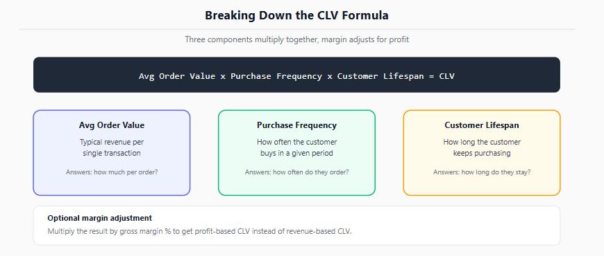
A breakdown of the CLV formula into average order value, purchase frequency, customer lifespan, and margin, with what each component answers

CLV (revenue-based) = Average Order Value x Purchase Frequency x Customer Lifespan
CLV (margin-based)  = CLV (revenue-based) x Gross Margin %

Each component needs its own definition before this formula produces a usable number. “Purchase frequency” needs a time window (orders per month, per year). “Customer lifespan” needs a definition of when a customer is considered to have stopped purchasing, which is itself a judgment call rather than a fixed threshold, since the right cutoff depends on the product’s typical purchase cadence.

Calculating Historic CLV With SQL

For Meridian Goods, the marketing team wants historic CLV computed per customer, using all transaction history to date. The calculation breaks into the same three components as the formula above.

-- Step 1: per-customer aggregates (PostgreSQL syntax)
WITH customer_orders AS (
    SELECT
        customer_id,
        COUNT(DISTINCT order_id) AS total_orders,
        SUM(order_total) AS total_revenue,
        MIN(order_date) AS first_order_date,
        MAX(order_date) AS last_order_date
    FROM orders
    GROUP BY customer_id
)

-- Step 2: derive average order value, tenure, and historic CLV
SELECT
    customer_id,
    total_orders,
    total_revenue,
    ROUND(total_revenue / NULLIF(total_orders, 0), 2) AS avg_order_value,
    DATE_PART('day', last_order_date - first_order_date) / 30.0 AS tenure_months,
    total_revenue AS historic_clv
FROM customer_orders;

total_revenue in the final column is historic CLV by definition: it is simply the sum of everything the customer has spent to date, which is why historic CLV requires no assumptions once the transaction data is clean. The DATE_PART() function used for tenure is PostgreSQL-specific; other engines compute a date difference differently (for example, DATEDIFF() in several warehouses), so this line needs adjusting before it runs unmodified elsewhere. The PostgreSQL aggregation functions documentation covers SUM, COUNT DISTINCT, and the other aggregates used in the first CTE.

To turn this into a segment-level or cohort-level average rather than a per-customer figure, wrap the query in an outer aggregation:

SELECT
    ROUND(AVG(historic_clv), 2) AS avg_historic_clv,
    COUNT(*) AS customer_count
FROM customer_clv;

If the goal is margin-based CLV rather than revenue-based, the same query needs a cost or margin field joined in before the final SUM(), since revenue alone overstates value for products with materially different margins across the catalog.

Calculating Historic CLV in Excel

The same calculation is achievable in Excel without SQL, using a transaction-level table with one row per order and SUMIFS and COUNTIFS to build the per-customer aggregates. Assuming columns for Customer ID, Order Date, and Order Total:

Total Revenue per customer:  =SUMIFS(OrderTotal, CustomerID, [@CustomerID])
Total Orders per customer:   =COUNTIFS(CustomerID, [@CustomerID])
Average Order Value:         =[@TotalRevenue] / [@TotalOrders]
First Order Date:            =MINIFS(OrderDate, CustomerID, [@CustomerID])
Last Order Date:             =MAXIFS(OrderDate, CustomerID, [@CustomerID])
Tenure (months):             =([@LastOrderDate] - [@FirstOrderDate]) / 30
Historic CLV:                =[@TotalRevenue]

A pivot table is usually a cleaner way to get to the per-customer summary than repeating SUMIFS and COUNTIFS down every row, particularly once the transaction table grows large enough that per-row formulas become slow to recalculate. As the transaction volume grows, performance in Excel may degrade compared to a database query, and the Excel specifications and limits page documents the current row and column limits if the dataset is approaching them. For teams that outgrow row-by-row Excel formulas on this kind of calculation, the Gradient Learnings comparison of pandas versus Excel covers where that switch typically becomes worthwhile.

Choosing the Right CLV Approach for Your Data

Historic CLV is not the right choice for every question. If the marketing team’s actual question is “what should we expect a brand-new customer to be worth,” a purely historic number for existing customers understates the answer, since it does not account for customers who are still early in their lifecycle and have not yet generated their full value.

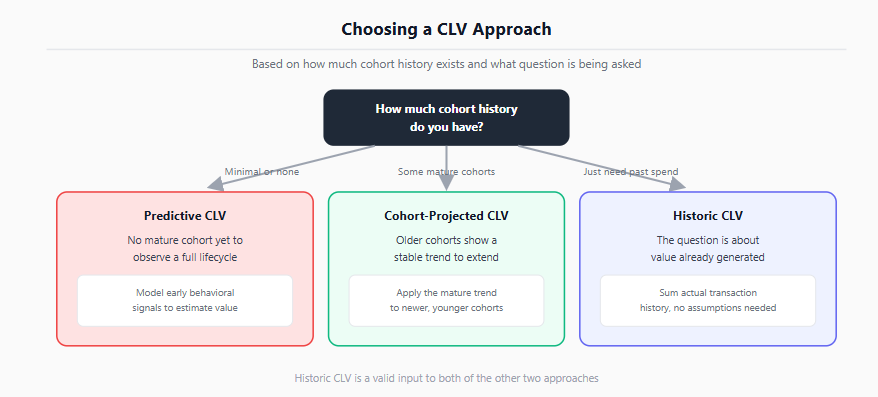
A decision framework for choosing between historic CLV, cohort-projected CLV, and predictive CLV based on data history length and the question being asked

For Meridian Goods specifically, if enough historical cohorts exist to see how spend and retention evolve over the first several months, a cohort-projected approach (taking the observed trend for cohorts that are further along and applying it to newer cohorts) gives a more forward-looking estimate without requiring a full predictive model. If the business is new enough that no cohort has reached a mature lifecycle yet, predictive CLV based on early behavioral signals (first-order size, category, acquisition channel) is generally the more appropriate next step, though it requires a modeling effort beyond a single query or spreadsheet.

Common Mistakes / Practical Checklist

• Reporting historic CLV as if it were a forecast. Historic CLV describes what has already happened; it does not project what a customer will spend in the future.

• Using revenue-based CLV to compare products or segments with materially different margins, which can make a low-margin, high-revenue segment look more valuable than a higher-margin segment with lower revenue.

• Averaging CLV across customers with very different tenures without noting that newer customers have had less time to generate value, which pulls the blended average down relative to what a mature customer eventually reaches.

• Applying a fixed “customer lifespan” number across every segment without checking whether purchase cadence actually differs by product line or acquisition channel.

• Reusing date-difference SQL syntax across engines without adjustment, since functions like DATE_PART(), DATEDIFF(), and TIMESTAMPDIFF() are not interchangeable.

• Skipping the margin adjustment when the decision being informed is about profitability (like acquisition spend) rather than pure revenue.

Where to Go From Here

This article assumes basic comfort with SQL aggregation and either SQL or Excel formulas for building per-customer summaries. If SQL is the gap, SQL for data analysts: essential skills is the right starting point. If the transaction data itself needs cleanup before any CLV calculation is reliable, for example inconsistent customer IDs or duplicate order records, cleaning messy data in Excel covers that groundwork. Framing a CLV number as an input to an acquisition-spend decision, rather than reporting it in isolation, follows the same discipline covered in the Gradient Learnings guide to solving a business problem with data. If the next step is presenting a CLV analysis in an interview setting, how to explain a data analyst project in an interview covers how to narrate that kind of analysis concisely.